Recognition: 2 theorem links
· Lean TheoremLearning stochastic multiscale models through normalizing flows
Pith reviewed 2026-05-12 03:42 UTC · model grok-4.3
The pith
Normalizing flows learn the invariant distribution of unobserved fast variables to derive reduced stochastic models from a single slow trajectory.
A machine-rendered reading of the paper's core claim, the machinery that carries it, and where it could break.
Core claim
The paper claims that the invariant distribution of the fast process can be parameterized by a normalizing flow and learned solely from one observed slow trajectory by optimizing the penalized likelihood induced by the stochastically averaged reduced model, while a variational flow approximates the parameter posterior for uncertainty quantification.
What carries the argument
Normalizing flow parameterization of the invariant density of the fast variables, inserted into the stochastic averaging formula for the reduced slow-scale SDE.
If this is right
- The reduced model can be learned from limited slow-only data while preserving the interaction between scales.
- Uncertainty in the learned parameters can be quantified scalably via variational inference with a second flow.
- The approach avoids both dense data requirements and grid-based PDE solvers common in Fokker-Planck methods.
- The framework yields effective dynamics that respect the original stochastic structure rather than generic dimensionality reduction.
Where Pith is reading between the lines
- The same flow-based reduction could be tested on real observational time series from biology or climate where fast variables are inaccessible.
- If the learned invariant distribution matches the true one, the method should reproduce both equilibrium and transient statistics of the slow variable at long times.
- The penalized likelihood objective might be extended to include additional physical constraints such as conservation laws without changing the flow architecture.
Load-bearing premise
The invariant distribution of the fast process can be recovered to sufficient accuracy from statistics of the slow trajectory alone, without any direct observations of the fast variables.
What would settle it
Generate a known multiscale SDE system, observe only the slow trajectory, apply the method, then compare the long-term statistics or transition densities of the learned reduced model against independent long simulations of the original full system; large systematic mismatch would falsify the claim.
Figures


read the original abstract
Many systems in physics, engineering, and biology exhibit multiscale stochastic dynamics, where low-dimensional slow variables evolve under the influence of high-dimensional fast processes. In practice, observations are often limited to a single trajectory of the slow component, while the fast dynamics remain unobserved, making statistical learning challenging. Approaches based on partial differential equations (PDE), such as Fokker-Planck formulations, aim to characterize the evolution of probability densities, typically requiring dense space-time data or grid-based solvers. In contrast, we adopt a trajectory-based perspective and develop a data-driven framework for learning effective stochastic dynamics from a single observed path. We model the dynamics by coupled multiscale stochastic differential equations (SDEs) and first obtain a principled model reduction through stochastic averaging. Unlike generic model reduction techniques such as PCA, this respects the dynamical structure of the original system and explicitly incorporates the interaction between slow and fast scales. A central challenge, however, is that the reduced model depends on the invariant distribution of the fast process, which is a solution to an intractable and often unknown PDE. We introduce a novel learning framework that parameterizes the invariant distribution using normalizing flows, enabling expressive density modeling in the latent fast-variable space. The flow is trained end-to-end by optimizing a penalized likelihood objective induced by the reduced stochastic dynamics. Furthermore, we develop a Bayesian variational inference procedure for uncertainty quantification, employing a second normalizing flow to approximate the posterior distribution over model parameters. This yields a scalable approach to capturing epistemic uncertainty in multiscale systems.
Editorial analysis
A structured set of objections, weighed in public.
Referee Report
Summary. The manuscript proposes a data-driven framework for learning reduced stochastic models of multiscale systems from a single observed trajectory of the slow variables. Stochastic averaging yields an effective SDE whose drift and diffusion depend on the invariant measure of the fast process; this measure is parameterized by a normalizing flow in the latent fast-variable space. The flow is trained end-to-end by optimizing a penalized likelihood induced by the reduced dynamics, and a second normalizing flow is used within variational inference to quantify posterior uncertainty over the model parameters.
Significance. If the central claims hold, the work would offer a scalable trajectory-based alternative to PDE-based methods for multiscale model reduction, allowing expressive density estimation of the fast-process invariant without direct observations or grid solvers. The end-to-end training and built-in uncertainty quantification via normalizing flows are notable strengths that could benefit applications in physics, biology, and engineering. The significance is reduced, however, by questions about whether the slow-scale likelihood can uniquely identify the invariant measure itself.
major comments (1)
- Abstract (central claim on learning the invariant distribution): The penalized likelihood is induced solely by the stochastically averaged SDE, whose coefficients are expectations of fast-scale functions against the invariant measure μ(y|x). Because this averaging map is not injective, distinct measures can produce identical reduced drift/diffusion and therefore identical likelihood values on the observed slow trajectory. Consequently, optimizing the normalizing-flow parameters cannot guarantee recovery of the true invariant; it only selects some measure whose averages match the slow-scale fit. This directly undermines the claim that the flow 'parameterizes the invariant distribution' and learns it from slow data alone.
minor comments (2)
- Abstract and method description: The specific form of the penalized likelihood objective, the manner in which expectations over the fast process are evaluated during training, and any regularization terms are only sketched at a high level; explicit equations would improve reproducibility and allow assessment of numerical stability.
- Notation: The dependence of the reduced coefficients on the flow parameters is not denoted explicitly (e.g., as functions of the flow parameters θ), which obscures how gradients flow through the averaging step in the end-to-end training.
Simulated Author's Rebuttal
We thank the referee for the careful reading and for identifying a key subtlety in the identifiability of the invariant measure. We have revised the manuscript to clarify the precise scope of our claims while preserving the core contribution of the end-to-end trajectory-based framework.
read point-by-point responses
-
Referee: Abstract (central claim on learning the invariant distribution): The penalized likelihood is induced solely by the stochastically averaged SDE, whose coefficients are expectations of fast-scale functions against the invariant measure μ(y|x). Because this averaging map is not injective, distinct measures can produce identical reduced drift/diffusion and therefore identical likelihood values on the observed slow trajectory. Consequently, optimizing the normalizing-flow parameters cannot guarantee recovery of the true invariant; it only selects some measure whose averages match the slow-scale fit. This directly undermines the claim that the flow 'parameterizes the invariant distribution' and learns it from slow data alone.
Authors: We agree that the stochastic averaging map is not injective in general, so the slow-scale likelihood does not uniquely identify the full invariant measure μ. The framework learns a normalizing-flow parameterization of a measure whose expectations against the relevant fast-scale functions reproduce the effective drift and diffusion coefficients consistent with the observed slow trajectory. This yields a useful reduced stochastic model even when the full density is not uniquely recoverable. We have revised the abstract, introduction, and discussion sections to state explicitly that the method recovers an effective invariant measure whose averages match the data, rather than claiming unique recovery of the true underlying distribution from slow data alone. Numerical experiments continue to show that the learned measure produces accurate reduced dynamics on the slow scale. revision: yes
Circularity Check
No significant circularity; derivation is self-contained
full rationale
The paper starts from multiscale SDEs, applies stochastic averaging to derive a reduced model whose coefficients are expectations against the fast-process invariant measure, then parameterizes that measure via normalizing flows and optimizes a penalized likelihood on the observed slow trajectory. This is standard parameter estimation using external techniques (stochastic averaging and flow-based density estimation) rather than any self-definitional loop, fitted input renamed as prediction, or load-bearing self-citation. No equations or steps in the provided description reduce the claimed result to its inputs by construction. The central claim retains independent content from the data-driven training procedure.
Axiom & Free-Parameter Ledger
free parameters (2)
- normalizing flow parameters
- reduced SDE model parameters
axioms (2)
- domain assumption The fast process possesses a well-defined invariant distribution
- domain assumption Stochastic averaging yields an accurate effective dynamics description from the multiscale SDEs
Lean theorems connected to this paper
-
IndisputableMonolith/Cost/FunctionalEquation.leanwashburn_uniqueness_aczel unclearWe introduce a novel learning framework that parameterizes the invariant distribution using normalizing flows... The flow is trained end-to-end by optimizing a penalized likelihood objective induced by the reduced stochastic dynamics.
-
IndisputableMonolith/Foundation/RealityFromDistinction.leanreality_from_one_distinction unclearthe reduced model depends on the invariant distribution of the fast process... π₀ is the unique stationary distribution of A₁
Reference graph
Works this paper leans on
-
[1]
Assyr Abdulle, Giacomo Garegnani, Grigorios A Pavliotis, Andrew M Stuart, and Andrea Zanoni. Drift estimation of multiscale diffusions based on filtered data.Foundations of Computational Mathematics, 23(1):33–84, 2023
work page 2023
-
[2]
Closed-form likelihood expansions for multivariate diffusions.Ann
Yacine Aït-Sahalia. Closed-form likelihood expansions for multivariate diffusions.Ann. Statist., 36(2):906–937, 2008
work page 2008
-
[3]
Approximate inference for continuous-time Markov processes
Cédric Archambeau and Manfred Opper. Approximate inference for continuous-time Markov processes. InBayesian time series models, pages 125–140. Cambridge Univ. Press, Cambridge, 2011
work page 2011
-
[4]
Jaya P. N. Bishwal.Parameter estimation in stochastic volatility models. Springer, Cham, 2022
work page 2022
-
[5]
Mogens Bladt and Michael Sø rensen. Simple simulation of diffusion bridges with application to likelihood inference for diffusions.Bernoulli, 20(2):645–675, 2014
work page 2014
-
[6]
On the approximate maximum likelihood estimation for diffusion processes.Ann
Jinyuan Chang and Song Xi Chen. On the approximate maximum likelihood estimation for diffusion processes.Ann. Statist., 39(6):2820–2851, 2011
work page 2011
-
[7]
Approximate inference in latent gaussian-markov models from continuous time observations
Botond Cseke, Manfred Opper, and Guido Sanguinetti. Approximate inference in latent gaussian-markov models from continuous time observations. In C. J. C. Burges, L. Bottou, M. Welling, Z. Ghahramani, and K. Q. Weinberger, editors,Advances in Neural Information Processing Systems 26, pages 971–979. Curran Associates, Inc., 2013
work page 2013
-
[8]
Likelihood inference for discretely observed nonlinear diffusions.Econometrica, 69(4):959–993, 2001
Ola Elerian, Siddhartha Chib, and Neil Shephard. Likelihood inference for discretely observed nonlinear diffusions.Econometrica, 69(4):959–993, 2001
work page 2001
-
[9]
Yves Frederix, Giovanni Samaey, and Dirk Roose. An analysis of noise propagation in the multiscale simulation of coarse fokker-planck equations.ESAIM: Mathematical Modelling and Numerical Analysis, 45(3):541–561, 2011
work page 2011
-
[10]
Siragan Gailus and Konstantinos Spiliopoulos. Discrete-time statistical inference for multiscale diffusions.Multiscale Modeling & Simulation, 16(4):1824–1858, 2018
work page 2018
-
[11]
A. Golightly and D. J. Wilkinson. Bayesian inference for nonlinear multivariate diffusion models observed with error.Comput. Statist. Data Anal., 52(3):1674–1693, 2008
work page 2008
-
[12]
Approximation capabilities of multilayer feedforward networks.Neural networks, 4(2):251–257, 1991
Kurt Hornik. Approximation capabilities of multilayer feedforward networks.Neural networks, 4(2):251–257, 1991
work page 1991
-
[13]
Iacus.Simulation and inference for stochastic differential equations
Stefano M. Iacus.Simulation and inference for stochastic differential equations. Springer Series in Statistics. Springer, New York, 2008. With R examples
work page 2008
-
[14]
Estimation of an ergodic diffusion from discrete observations.Scand
Mathieu Kessler. Estimation of an ergodic diffusion from discrete observations.Scand. J. Statist., 24(2):211–229, 1997
work page 1997
-
[15]
Universal approximation with deep narrow networks
Patrick Kidger and Terry Lyons. Universal approximation with deep narrow networks. In Conference on learning theory, pages 2306–2327. PMLR, 2020
work page 2020
-
[16]
Maximum-likelihood estimation for diffusion processes via closed-form density expansions.Ann
Chenxu Li. Maximum-likelihood estimation for diffusion processes via closed-form density expansions.Ann. Statist., 41(3):1350–1380, 2013
work page 2013
-
[17]
George Papamakarios, Eric Nalisnick, Danilo Jimenez Rezende, Shakir Mohamed, and Balaji Lakshminarayanan. Normalizing flows for probabilistic modeling and inference.Journal of Machine Learning Research, 22(57):1–64, 2021
work page 2021
-
[18]
Grigorios A Pavliotis, Yvo Pokern, and Andrew M Stuart. Parameter estimation for multiscale diffusions: an overview.Statistical methods for stochastic differential equations, 124:429, 2012
work page 2012
-
[19]
Parameter estimation for multiscale diffusions.Journal of Statistical Physics, 127(4):741–781, 2007
Grigorios A Pavliotis and AM Stuart. Parameter estimation for multiscale diffusions.Journal of Statistical Physics, 127(4):741–781, 2007
work page 2007
-
[20]
Grigorios A. Pavliotis and Andrew M. Stuart.Multiscale methods, volume 53 ofTexts in Applied Mathematics. Springer, New York, 2008. Averaging and homogenization. 10
work page 2008
-
[21]
Lukas Pichler, Arif Masud, and Lawrence A Bergman. Numerical solution of the fokker– planck equation by finite difference and finite element methods—a comparative study. In Computational Methods in Stochastic Dynamics: Volume 2, pages 69–85. Springer, 2013
work page 2013
-
[22]
Variational inference with normalizing flows
Danilo Rezende and Shakir Mohamed. Variational inference with normalizing flows. In International conference on machine learning, pages 1530–1538. PMLR, 2015
work page 2015
-
[23]
G. O. Roberts and O. Stramer. On inference for partially observed nonlinear diffusion models using the Metropolis-Hastings algorithm.Biometrika, 88(3):603–621, 2001
work page 2001
-
[24]
Timo Sprekeler, Endre Süli, and Zhiwen Zhang. Finite element approximation of stationary fokker–planck–kolmogorov equations with application to periodic numerical homogenization. SIAM Journal on Numerical Analysis, 63(3):1315–1343, 2025
work page 2025
-
[25]
Cédric Villani et al.Optimal transport: old and new, volume 338. Springer, 2009
work page 2009
-
[26]
Whitaker, Andrew Golightly, Richard J
Gavin A. Whitaker, Andrew Golightly, Richard J. Boys, and Chris Sherlock. Bayesian inference for diffusion-driven mixed-effects models.Bayesian Anal., 12(2):435–463, 2017
work page 2017
-
[27]
Yunfei Yang, Zhen Li, and Yang Wang. On the capacity of deep generative networks for approximating distributions.Neural networks, 145:144–154, 2022
work page 2022
-
[28]
Estimation for diffusion processes from discrete observation.J
Nakahiro Yoshida. Estimation for diffusion processes from discrete observation.J. Multivariate Anal., 41(2):220–242, 1992. A Theoretical details and results A.1 Stochastic averaging of fast-slow sde system Proof of Theorem 3.2.Notice thatY (n)(·) Law =Y(n·)whereYsatisfies the SDE: dY(t) =β Y(t) dt+α Y(t) d ˜W(t).(20) Fixp >1. By Itô’s lemma V p(Y(t)) =V p...
work page 1992
-
[29]
+y 4 4 . The cubic structure in the numerator induces a double-well behavior in the effective averaged dynamics, while the denominator introduces a highly nonlinear dependence on the fast variables. Experimental Design:Synthetic observations are generated by simulating the corresponding multiscale slow–fast SDE system using Euler–Maruyama discretization o...
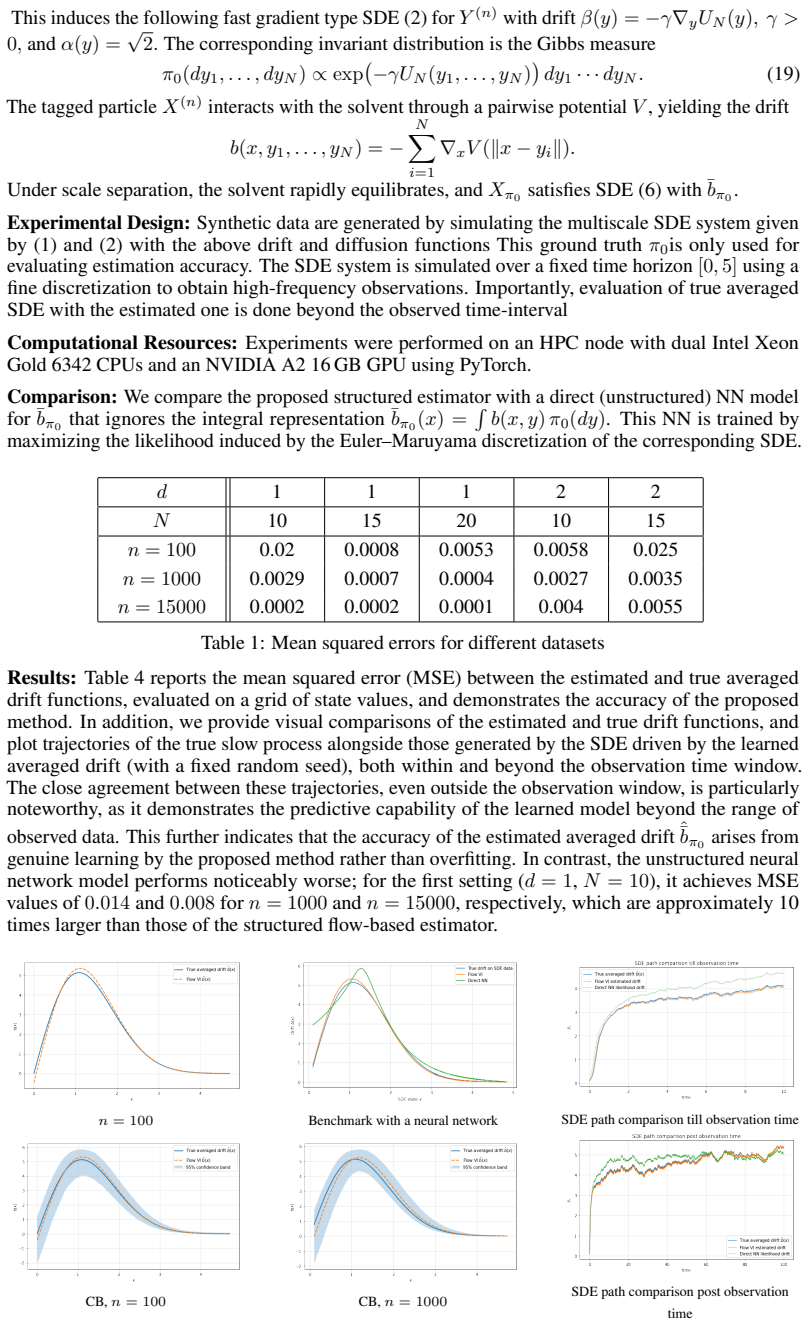
discussion (0)
Sign in with ORCID, Apple, or X to comment. Anyone can read and Pith papers without signing in.