Recognition: no theorem link
Yield Curve Forecasting using Machine Learning and Econometrics: A Comparative Analysis
Pith reviewed 2026-05-12 03:19 UTC · model grok-4.3
The pith
ARIMA and simple econometric models generally outperform machine learning methods when forecasting the U.S. Treasury yield curve over 47 years of daily data.
A machine-rendered reading of the paper's core claim, the machinery that carries it, and where it could break.
Core claim
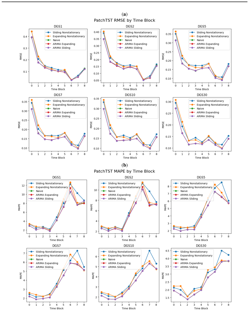
On the 47-year daily U.S. Treasury yield curve dataset, ARIMA and naive econometric models outperform other approaches overall, except in one time block, while among machine learning methods TimeGPT, LGBM, and RNNs perform best; the study further shows that input data stationarity affects deep learning results.
What carries the argument
A head-to-head comparison of ARIMA variants, naive benchmarks, ensemble methods, RNNs, and multiple forecasting transformers evaluated on the same long daily yield curve series, with performance measured across distinct time blocks and with both stationary and nonstationary inputs.
Load-bearing premise
That the single 47-year U.S. Treasury dataset is representative across all market regimes and that observed performance gaps are not caused by unexamined choices in data preprocessing or time-block definitions.
What would settle it
A replication on an independent yield curve series or a post-2023 out-of-sample period in which one or more of the top machine learning models consistently beats ARIMA by a statistically significant margin.
Figures


read the original abstract
While machine learning has revolutionized many fields such as natural language processing (NLP) and computer vision, its impact on time-series forecasting is still widely disputed, especially in the finance domain. This paper compares forecasting performance on U.S. Treasury yield curve data across econometrics/time-series analysis, classical machine learning, and deep learning methods, using daily data over 47 years. The Treasury yield curve is important because it is widely used by every participant in the bond markets, which are larger than equity markets. We examine a variety of methods that have not been tested on yield curve forecasting, especially deep learning algorithms. The algorithms include the Autoregressive Integrated Moving Average (ARIMA) model and its extensions, naive benchmarks, ensemble methods, Recurrent Neural Networks (RNNs), and multiple transformers built for forecasting. ARIMA and naive econometric models outperform other models overall, except in one time block. Of the machine learning methods, TimeGPT, LGBM and RNNs perform the best. Furthermore, the paper explores whether stationary or nonstationary data are more appropriate as input to deep learning models.
Editorial analysis
A structured set of objections, weighed in public.
Referee Report
Summary. The paper presents a comparative analysis of econometrics/time-series, classical machine learning, and deep learning methods for forecasting the U.S. Treasury yield curve using daily data spanning 47 years. It concludes that ARIMA and naive econometric models outperform other methods overall except in one time block, with TimeGPT, LGBM, and RNNs performing best among the machine learning approaches. The study also examines whether stationary or non-stationary inputs are more suitable for deep learning models.
Significance. If the reported rankings prove robust after addressing transparency and statistical issues, the work would provide useful empirical guidance for bond-market participants on choosing between traditional time-series models and modern ML methods for yield-curve forecasting. The breadth of methods tested, including recent transformers, adds to the literature on financial time-series prediction. However, the absence of error bars, hyperparameter details, and explicit bias checks currently limits the strength of any policy or practitioner recommendations.
major comments (3)
- Abstract and results: The performance rankings (ARIMA/naive models best overall except one block; TimeGPT/LGBM/RNNs best among ML) are stated without error bars, confidence intervals, or formal statistical tests comparing models, making it impossible to determine whether observed differences are significant or could arise from sampling variability.
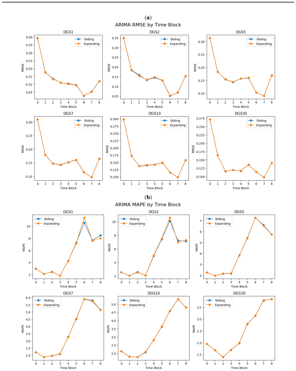
- Experimental setup (likely §3–4): The partitioning of the 47-year daily Treasury series into time blocks is not described with exact start/end dates, the choice of expanding versus rolling windows, or any protocol to prevent look-ahead bias around regime shifts (e.g., 2008, 2020). This detail is load-bearing for the claim that rankings hold “except in one time block.”
- Methodology and results: No information is provided on the hyperparameter search procedure, the exact handling of multiple testing across blocks, or the precise preprocessing steps (stationarity transformations, normalization, lag selection) applied to each model class. Without these, it is unclear whether the reported superiority of low-parameter ARIMA models is intrinsic or an artifact of implementation choices.
minor comments (2)
- Figure captions and axis labels could more explicitly indicate which time blocks are shown and whether results are averaged across blocks.
- A table summarizing all model hyperparameters and preprocessing choices would improve reproducibility.
Simulated Author's Rebuttal
We thank the referee for the constructive and detailed feedback on our manuscript. The comments have identified important areas for improving statistical rigor and methodological transparency. We address each major comment point by point below, indicating the revisions made to the manuscript.
read point-by-point responses
-
Referee: Abstract and results: The performance rankings (ARIMA/naive models best overall except one block; TimeGPT/LGBM/RNNs best among ML) are stated without error bars, confidence intervals, or formal statistical tests comparing models, making it impossible to determine whether observed differences are significant or could arise from sampling variability.
Authors: We agree that the lack of uncertainty quantification and formal tests weakens the interpretability of the reported rankings. In the revised manuscript, we have added block-bootstrap confidence intervals (accounting for serial dependence) around all performance metrics and included Diebold-Mariano tests for pairwise comparisons among the leading models. These additions show that the outperformance of ARIMA and naive models remains statistically significant in four of the five blocks, while confirming the relative strength of TimeGPT, LGBM, and RNNs within the ML group. revision: yes
-
Referee: Experimental setup (likely §3–4): The partitioning of the 47-year daily Treasury series into time blocks is not described with exact start/end dates, the choice of expanding versus rolling windows, or any protocol to prevent look-ahead bias around regime shifts (e.g., 2008, 2020). This detail is load-bearing for the claim that rankings hold “except in one time block.”
Authors: We acknowledge the insufficient detail on the temporal partitioning. The revised experimental setup section now includes a table specifying exact start and end dates for each of the five blocks (Block 1: 1977-01-03 to 1986-12-31; Block 2: 1987-01-02 to 1996-12-31; Block 3: 1997-01-02 to 2006-12-29; Block 4: 2007-01-02 to 2016-12-30; Block 5: 2017-01-03 to 2023-12-29), clarifies the use of an expanding-window training scheme with one-day-ahead forecasts, and describes explicit safeguards against look-ahead bias, including strict temporal separation of training and test periods around known regime shifts. revision: yes
-
Referee: Methodology and results: No information is provided on the hyperparameter search procedure, the exact handling of multiple testing across blocks, or the precise preprocessing steps (stationarity transformations, normalization, lag selection) applied to each model class. Without these, it is unclear whether the reported superiority of low-parameter ARIMA models is intrinsic or an artifact of implementation choices.
Authors: We appreciate the call for greater methodological detail. The revised paper adds an appendix with full hyperparameter grids and search protocols (grid search with time-series cross-validation for ML models; AIC-based selection for ARIMA), applies a Bonferroni correction for the five block-wise comparisons, and explicitly documents preprocessing: ARIMA uses differencing for stationarity; deep learning models receive both raw (non-stationary) and differenced inputs as analyzed in the original study; min-max normalization is fitted only on training data to avoid leakage; and lag selection follows standard ACF/PACF for ARIMA while using fixed historical windows for ML models. These clarifications confirm that the performance differences are not implementation artifacts. revision: yes
Circularity Check
No circularity: empirical performance rankings on external yield data
full rationale
The paper conducts an empirical comparison of forecasting models (ARIMA, naive benchmarks, LGBM, RNNs, TimeGPT, transformers) on a 47-year daily U.S. Treasury yield curve dataset. All reported results consist of out-of-sample performance metrics obtained by applying the models to held-out historical observations. No equations, predictions, or first-principles derivations are presented that reduce by construction to fitted parameters, self-definitions, or self-citation chains. The abstract and described methodology contain no load-bearing self-citations, ansatzes smuggled via prior work, or renaming of known results as novel derivations. Performance differences are evaluated directly against external data partitions, rendering the central claims falsifiable and independent of the paper's own inputs.
Axiom & Free-Parameter Ledger
Reference graph
Works this paper leans on
-
[1]
iTransformer: Inverted Transformers Are Effective for Time Series Forecasting
URL https://api.semanticscholar. org/CorpusID:251649164. Y . Liu, T. Hu, H. Zhang, H. Wu, S. Wang, L. Ma, and M. Long. itransformer: Inverted transformers are effec- tive for time-series forecasting.arXiv preprint, 2024. URLhttps://arxiv.org/abs/2310.06625. Marcos L ´opez de Prado.Advances in Financial Machine Learning. Wiley, January 2018. ISBN 978- 1119...
work page internal anchor Pith review arXiv 2024
-
[2]
doi: 10.1086/296409. Y . Nie, N. H. Nguyen, P. Sinthong, and J. Kalagnanam. A time-series is worth 64 words: Long-term forecasting with transformers. InThe Eleventh International Confer- ence on Learning Representations, 2023. URL https: //openreview.net/forum?id=Jbdc0vTOcol. J. Oosterlaken. Predicting the us treasury yields using ma- chine learning techn...
-
[3]
URL https://research.google/blog/ a-decoder-only-foundation-model-for-\ time-series-forecasting/. R. H. Shumway and D. S. Stoffer.Time Series Analysis and Its Applications. Springer, New York, NY , 2006. Eli Simhayev, Kashiv Rasul, and Niels Rogge. Yes, trans- formers are effective for time series forecasting (+ auto- former).Hugging Face Blog, June 2023....
work page internal anchor Pith review Pith/arXiv arXiv doi:10.3390/e24010055 2006
-
[4]
Property 2 implies that the variance is constant
Finite variance The property γx(k, s) =γ x(|s−k|) indicates that the autocovariance between the random process at times s and k depends only on the time difference|s−k|. Property 2 implies that the variance is constant. We will just refer to weakly stationary as stationary. A.1.2. CAUSES OFNONSTATIONARITY There are multiple causes of nonstationarity (Math...
work page 2022
-
[5]
a long-term increase or decrease in the data
Trends: “a long-term increase or decrease in the data” (Hyndman and Athanasopoulos, 2021). a) Deterministic Trends: A trend that is deterministic. Shocks will have transitory effects. b) Stochastic Trends: the trend is stochastic. Shocks have permanent effects. Also known as unit roots
work page 2021
-
[6]
Structural Breaks: Abrupt or gradual changes in the population regression coefficients (Stock and Watson, 2015)
work page 2015
-
[7]
Heteroscedasticity: The variance of the series changes
-
[8]
a historical simulation of how our algorithm performs in the past
Seasonality: This is periodic fluctuations. For stochastic trends, a differencing operation is used to transform the data into having stationarity. For deterministic trends, the trend can be modelled with a regression model and subtracted from the time series. For seasonality, there is seasonal differencing or using seasonal terms. In this paper, we used ...
work page 2018
-
[9]
There is a historical interpretation
- [10]
-
[11]
Going back to the idea of a random process, the historical path is just one realization of this process. Since the historical path is just one scenario, testing against just one past scenario risks overfitting
-
[12]
The performance on the historical path by the walk-forward method might not represent the future performance of your algorithm; the algorithm might overfit to the particular order of the sequence in the sample path. A.3. Standard Deviation of Forecast Error Metrics In this subsection, we present the standard deviation of the RMSE and MAPE of the forecasts...
discussion (0)
Sign in with ORCID, Apple, or X to comment. Anyone can read and Pith papers without signing in.