arxiv: 2605.11607 · v1 · submitted 2026-05-12 · 📊 stat.ML · cs.AI· cs.LG

Recognition: 2 theorem links

· Lean Theorem

Exact Stiefel Optimization for Probabilistic PLS: Closed-Form Updates, Error Bounds, and Calibrated Uncertainty

Haoran Hu, Xingce Wang

Pith reviewed 2026-05-13 01:17 UTC · model grok-4.3

classification 📊 stat.ML cs.AIcs.LG

keywords probabilistic partial least squaresStiefel manifold optimizationnoise-subspace estimationfinite-sample error boundscalibrated uncertaintymulti-omics datatwo-view learningorthogonal constraints

0 comments

The pith

A noise-subspace estimator for probabilistic partial least squares attains a signal-strength-independent finite-sample rate that matches the minimax lower bound, while the full-spectrum estimator is inconsistent.

A machine-rendered reading of the paper's core claim, the machinery that carries it, and where it could break.

The paper develops an end-to-end fitting procedure for probabilistic partial least squares that pre-estimates noise from the complement of the signal subspace and then performs exact optimization of the constrained likelihood on the Stiefel manifold. This produces closed-form updates together with error bounds showing that the noise estimator's leading term does not depend on signal strength and meets the minimax rate. The same pipeline supplies block-structured Fisher standard errors and yields prediction intervals with near-nominal coverage on synthetic high-noise data and real multi-omics benchmarks without any post-hoc adjustment. A reader would care because the method removes the coupling between noise and signal parameters that arises in joint EM or penalty-based schemes while delivering native calibrated uncertainty for interpretable two-view latent-factor models.

Core claim

Under the identifiable parameterization with fixed scalar noise, the combination of noise-subspace pre-estimation and exact Stiefel-manifold optimization yields closed-form parameter updates, a leading finite-sample error rate for the noise estimator that is independent of signal strength and matches a minimax lower bound, and inconsistency of the corresponding full-spectrum estimator; the framework further provides closed-form standard errors via block-structured Fisher analysis and extends to sub-Gaussian data through optional Gaussianization.

What carries the argument

exact Stiefel-manifold optimization of the constrained likelihood after noise-subspace pre-estimation

If this is right

Closed-form updates replace iterative joint EM or interior-point penalty methods for loadings and scores.
Standard errors follow directly from the block-structured Fisher information without additional approximation.
Prediction intervals achieve near-nominal coverage on high-noise synthetic settings and on TCGA-BRCA and PBMC CITE-seq data without recalibration.
Point accuracy reaches Ridge levels at low rank while cross-view prediction matches or exceeds existing methods.

Where Pith is reading between the lines

These are editorial extensions of the paper, not claims the author makes directly.

The separation of noise and signal subspaces could be exploited in other orthogonal latent-variable models to stabilize variance estimation.
The optional Gaussianization step indicates the method can be applied to non-Gaussian two-view data typical in single-cell genomics.
Closed-form standard errors simplify propagation of uncertainty into downstream multi-omics tasks such as pathway analysis.

Load-bearing premise

The data follow the identifiable two-view model with a single fixed scalar noise variance, and the noise subspace separates cleanly from the signal subspace.

What would settle it

Data generated from the model in which the empirical convergence rate of the noise-subspace estimator increases with signal strength, or in which the full-spectrum estimator remains consistent.

Figures

Figures reproduced from arXiv: 2605.11607 by Haoran Hu, Xingce Wang.

**Figure 2.** Figure 2: Empirical speedup (wall-clock ratio of matrix-form to scalar-form likelihood evaluation) [PITH_FULL_IMAGE:figures/full_fig_p026_2.png] view at source ↗

**Figure 3.** Figure 3: Single-run convergence trajectories in the canonical synthetic low-noise setting ( [PITH_FULL_IMAGE:figures/full_fig_p027_3.png] view at source ↗

**Figure 4.** Figure 4: Synthetic verification of Theorem 1 under fixed noise level σ 2 e = 0.5: absolute noiseestimation error |σˆ 2 e − σ 2 e | versus signal strength s ∈ {1, 2, 5, 10, 20} (log-scale x-axis). Error bars are Monte Carlo standard errors over M = 80 matched-seed runs; the dashed line is the leading bound in Eq. (5). interpreted as a property of the fixed-noise PPLS framework rather than of one optimizer only. Rel… view at source ↗

**Figure 5.** Figure 5: Downstream sensitivity to rank misspecification in the synthetic high-noise setting [PITH_FULL_IMAGE:figures/full_fig_p029_5.png] view at source ↗

**Figure 6.** Figure 6: MSE–calibration Pareto views on both real-data benchmarks: (a) TCGA-BRCA and [PITH_FULL_IMAGE:figures/full_fig_p031_6.png] view at source ↗

**Figure 7.** Figure 7: Noise-estimation ablation (M = 50 Monte Carlo trials, σ 2 e = 0.5): (a) mean absolute estimation error vs. dimension p (fixed N = 2000); (b) vs. sample size N (fixed p= 200). Error bars show Monte Carlo standard errors. The full-spectrum estimator (Hu 2025) suffers from a O(r/p) bias floor, while the noise-subspace estimator (ours) is essentially unbiased. inverse normal transform (Rank-INT) [PITH_FULL_IM… view at source ↗

**Figure 8.** Figure 8: Selective prediction on CITE-seq: retained-subset MSE versus retained ratio [PITH_FULL_IMAGE:figures/full_fig_p054_8.png] view at source ↗

**Figure 9.** Figure 9: Recovery plots for C (components 1–3) in the simulation setting of Section 6.3.1. Identifiability-preserving ordering. After convergence of each start, components are reordered so that θ 2 t,π(1)bπ(1) ≥ · · · ≥ θ 2 t,π(r) bπ(r) . Multi-start and warm start. Each start samples W, C via random QR and initializes Σt = B = Ir, σ 2 h = 0.01. One optional warm start uses top singular vectors of training cross-c… view at source ↗

**Figure 10.** Figure 10: Recovery plots for W (components 1–3) in the simulation setting of Section 6.3.1. D.3 Licenses for existing assets Datasets. • TCGA-BRCA Multi-Omics [Demharter and Stentoft, 2020]: Kaggle distribution under CC BY-NC-SA 4.0. • PBMC CITE-seq reference [Hao et al., 2021]: public SeuratData/10x resources for academic research. Software. • Pymanopt [Townsend et al., 2016]: BSD 3-Clause. • Manopt [Boumal et al.… view at source ↗

read the original abstract

Probabilistic partial least squares (PPLS) is a central likelihood-based model for two-view learning when one needs both interpretable latent factors and calibrated uncertainty. Building on the identifiable parameterization of Bouhaddani et al.\ (2018), existing fitting pipelines still face two practical bottlenecks: noise--signal coupling under joint EM/ECM updates and nontrivial handling of orthogonality constraints. Following the fixed-noise scalar-likelihood line of Hu et al.\ (2025), we develop an end-to-end framework that combines noise pre-estimation, constrained likelihood optimization, and prediction calibration in one pipeline. Relative to Hu et al.\ (2025), we replace full-spectrum noise averaging with noise-subspace estimation and replace interior-point penalty handling with exact Stiefel-manifold optimization. The noise-subspace estimator attains a signal-strength-independent leading finite-sample rate and matches a minimax lower bound, while the full-spectrum estimator is shown to be inconsistent under the same model. We further extend the framework to sub-Gaussian settings via optional Gaussianization and provide closed-form standard errors through a block-structured Fisher analysis. Across synthetic high-noise settings and two multi-omics benchmarks (TCGA-BRCA and PBMC CITE-seq), the method achieves near-nominal coverage without post-hoc recalibration, reaches Ridge-level point accuracy on TCGA-BRCA at rank $r=3$, matches or exceeds PO2PLS on cross-view prediction while providing native calibrated uncertainty, and improves stability of parameter recovery.

Editorial analysis

A structured set of objections, weighed in public.

Desk editor's note, referee report, simulated authors' rebuttal, and a circularity audit. Tearing a paper down is the easy half of reading it; the pith above is the substance, this is the friction.

Desk Editor's Note private letter to a colleague

Exact Stiefel closed-form updates and a noise-subspace estimator with claimed signal-independent rates are the concrete additions, but the separation from signal subspace still needs an explicit gap condition to back the minimax claim.

read the letter

The paper replaces interior-point penalties with exact Stiefel-manifold updates and swaps full-spectrum noise averaging for a noise-subspace estimator. These changes sit on top of the Bouhaddani identifiable parameterization and the authors' own fixed-noise scalar likelihood. The new pieces are the closed-form updates, the signal-strength-independent finite-sample rate for the noise subspace, the inconsistency proof for the full-spectrum estimator, and the block-structured Fisher standard errors. Experiments on synthetic high-noise data plus TCGA-BRCA and PBMC CITE-seq show near-nominal coverage without recalibration and prediction accuracy that reaches Ridge levels at low rank while matching or beating PO2PLS on cross-view tasks. That combination of exact optimization and native calibration is useful for the multi-omics niche where calibrated uncertainty matters. The main soft spot is the separation assumption. The headline rate and minimax-matching claims rest on the noise subspace separating cleanly from the signal subspace, yet the abstract gives no explicit eigenvalue-gap condition or pre-estimation requirement that would guarantee this when signal strength varies. If separation fails for weaker signals, the claimed independence and lower-bound match would not hold. The derivations for the rates and the inconsistency result are not visible in the abstract, so their tightness remains to be checked in the full proofs. This work is for readers already using probabilistic PLS in genomics or similar two-view settings who want better fitting routines and built-in uncertainty. It refines an existing framework rather than introducing a new model. I would send it to peer review. The technical claims on rates, inconsistency, and manifold optimization are worth a detailed referee check even if the separation condition needs tightening.

Referee Report

1 major / 1 minor

Summary. The paper develops an end-to-end framework for probabilistic partial least squares (PPLS) that combines noise pre-estimation, exact Stiefel-manifold optimization for the loading matrices, and prediction calibration. Building on the identifiable parameterization of Bouhaddani et al. (2018) and the fixed-noise scalar-likelihood model of Hu et al. (2025), it replaces full-spectrum noise averaging with a noise-subspace estimator that attains a signal-strength-independent leading finite-sample rate matching a minimax lower bound, shows inconsistency of the full-spectrum estimator, extends the approach to sub-Gaussian data via optional Gaussianization, derives closed-form standard errors via block-structured Fisher information, and reports competitive point accuracy, stability, and near-nominal coverage on synthetic high-noise data and two multi-omics benchmarks (TCGA-BRCA, PBMC CITE-seq).

Significance. If the finite-sample bounds and separation claims hold, the work would provide a theoretically grounded, computationally exact alternative to EM/ECM pipelines for PPLS, with the noise-subspace rate independence and minimax matching offering a clear advantage in high-noise regimes and the native calibration removing the need for post-hoc recalibration. The closed-form updates and Fisher-based standard errors are practical strengths for applied multi-view settings.

major comments (1)

[Abstract] Abstract and model setup: the headline claim that the noise-subspace estimator attains a signal-strength-independent leading finite-sample rate and matches the minimax lower bound rests on the assumption that this estimator separates cleanly from the signal subspace. No explicit eigenvalue-gap condition (or finite-sample guarantee on separation given the pre-estimated noise variance) is stated to ensure the separation holds when signal strength varies, which is load-bearing for both the rate-independence result and the lower-bound matching.

minor comments (1)

[Abstract] Abstract: the compound term 'noise--signal' uses a double dash that should be rendered as a single hyphen or en-dash for 'noise-signal coupling'.

Simulated Author's Rebuttal

1 responses · 0 unresolved

We thank the referee for the careful reading and for highlighting the need for an explicit separation condition. We address the comment below and will revise the manuscript to strengthen the presentation of the finite-sample results.

read point-by-point responses

Referee: [Abstract] Abstract and model setup: the headline claim that the noise-subspace estimator attains a signal-strength-independent leading finite-sample rate and matches the minimax lower bound rests on the assumption that this estimator separates cleanly from the signal subspace. No explicit eigenvalue-gap condition (or finite-sample guarantee on separation given the pre-estimated noise variance) is stated to ensure the separation holds when signal strength varies, which is load-bearing for both the rate-independence result and the lower-bound matching.

Authors: We agree that the rate-independence and minimax-matching claims for the noise-subspace estimator require a clean separation from the signal subspace, and that this separation must be guaranteed uniformly over a range of signal strengths. The current manuscript relies on the identifiable parameterization of Bouhaddani et al. (2018) together with the fixed-noise scalar-likelihood model of Hu et al. (2025) and the consistency of the pre-estimated noise variance; under these conditions the leading eigenvectors of the noise-subspace estimator are separated from the signal subspace with high probability once the noise variance is estimated at the stated rate. However, we acknowledge that an explicit eigenvalue-gap assumption (or a finite-sample probabilistic guarantee on the gap given the pre-estimated noise level) is not stated in the abstract or model section. In the revision we will add a precise statement of the required gap condition (adapted from the perturbation analysis in the supplementary material) and include a short lemma showing that the pre-estimated noise variance yields the necessary separation with probability 1-o(1) uniformly over signal strengths above a fixed threshold. This will make the load-bearing assumption fully explicit without altering the existing proofs. revision: yes

Circularity Check

0 steps flagged

No significant circularity in the claimed derivations

full rationale

The manuscript cites Hu et al. (2025) for the fixed-noise scalar-likelihood model and Bouhaddani et al. (2018) for the identifiable parameterization. However, the new technical contributions, including the exact Stiefel-manifold optimization, the noise-subspace estimator with its finite-sample rate and minimax matching, the inconsistency result for the full-spectrum estimator, the block-structured Fisher analysis for standard errors, and the extensions to sub-Gaussian settings, are developed within this paper. No quoted step shows a result being equivalent to the inputs by construction or the central claims reducing solely to self-citation without independent content. The derivation chain appears self-contained against the stated model assumptions.

Axiom & Free-Parameter Ledger

0 free parameters · 2 axioms · 0 invented entities

The work inherits the core PPLS likelihood and identifiability constraints from Bouhaddani et al. (2018) and the fixed-noise scalar model from Hu et al. (2025); no new free parameters or invented entities are introduced in the abstract.

axioms (2)

domain assumption Identifiable parameterization of Bouhaddani et al. (2018)
Used as the base model for all subsequent optimization and bounds.
domain assumption Fixed-noise scalar-likelihood model of Hu et al. (2025)
Underpins the separation of noise pre-estimation from signal optimization.

pith-pipeline@v0.9.0 · 5573 in / 1334 out tokens · 31170 ms · 2026-05-13T01:17:03.372342+00:00 · methodology

discussion (0)

Lean theorems connected to this paper

Citations machine-checked in the Pith Canon. Every link opens the source theorem in the public Lean library.

IndisputableMonolith/Cost/FunctionalEquation.lean washburn_uniqueness_aczel unclear
The scalar expansion ... ln(det Σ) = (p-r) ln σ²_e + ... + Σ ln D_i ... with D_i = (σ²_f + σ²_h)(θ²_ti + σ²_e) + b²_i θ²_ti σ²_e

Reference graph

Works this paper leans on

16 extracted references · 16 canonical work pages

[1]

Scalar likelihood method for probabilistic partial least squares model with rank n update

Haoran Hu, Xingce Wang, Zhongke Wu, Shilei Du, Yuhe Zhang, and Quansheng Liu. Scalar likelihood method for probabilistic partial least squares model with rank n update. In Proceedings of the 28th European Conference on Artificial Intelligence (ECAI 2025),

work page 2025
[2]

Mauck, Yuhan Hao, Marlon Stoeckius, Peter Smibert, and Rahul Satija

Tim Stuart, Andrew Butler, Paul Hoffman, Christoph Hafemeister, Efthymia Papalexi, William M. Mauck, Yuhan Hao, Marlon Stoeckius, Peter Smibert, and Rahul Satija. Compre- hensive integration of single-cell data.Cell, 177(7):1888–1902,

work page 1902
[3]

37 A Supplementary Proofs Notation.We use standard asymptotic notation throughout: aN ≲b N means aN ≤Cb N for some absolute constant C > 0; aN ≍b N means cbN ≤a N ≤Cb N for absolute constants 0 < c < C ; aN ≪b N means aN /bN → 0; OP (·) denotes the usual stochastic boundedness (in probability). The symbol C > 0 denotes a generic absolute constant that may...

work page 2025
[4]

Since ˆθN minimizesL, η≤ L ∞(ˆθN)− L ∞(θ0)≤2 sup θ∈K0 |L(θ)− L ∞(θ)|, so Pr( ˆθN ∈K ε)→0

Step 3 (Consistency).For any ε > 0, define Kε = {θ∈K 0 : ∥θ−θ 0∥ ≥ε} and η= inf Kε L∞(θ)− L ∞(θ0)>0. Since ˆθN minimizesL, η≤ L ∞(ˆθN)− L ∞(θ0)≤2 sup θ∈K0 |L(θ)− L ∞(θ)|, so Pr( ˆθN ∈K ε)→0. A.3 Asymptotic normality proof details Proof. Chart construction.We work in local coordinates on Mr = St(p, r) ×St (q, r) ×R 2r+1 ++ . For W∈St (p, r), we use exponen...

work page 2023
[5]

Mapping back through the chart diffeomorphism yields the stated limit for ˆθN [van der Vaart, 1998, Newey and McFadden, 1994, Theorem 5.39]

d− → N(0,I(θ0)−1). Mapping back through the chart diffeomorphism yields the stated limit for ˆθN [van der Vaart, 1998, Newey and McFadden, 1994, Theorem 5.39]. A.4 Verification details for optimization convergence Proof. The standard convergence theorem [Absil et al., 2008, Theorem 4.3.1] requires: (R1) objective C1 on manifold, (R2) iterates in a compact...

work page 1998
[6]

If s⋆ ≤ 0, then ∂ℓi/∂s does not change sign on s > 0 (it is non-negative throughout or non-positive throughout), so the minimum of ℓi on s > 0 is achieved as s→ 0+

If s⋆ > 0, it is the conditional maximizer. If s⋆ ≤ 0, then ∂ℓi/∂s does not change sign on s > 0 (it is non-negative throughout or non-positive throughout), so the minimum of ℓi on s > 0 is achieved as s→ 0+. In this case, we clip to s = ε for a small ε > 0, which approximates the boundary minimizer while maintaining strict positivity for numerical stabil...

work page 2018
[7]

If ˆr > r0, surplus loading directions are pushed toward the noise subspace and their associated strengths satisfy θ2 t,k → 0 for redundant components

B.4 Effect of rank misspecification on inference Suppose the fitted rank ˆrdiffers from the true rank r0. If ˆr > r0, surplus loading directions are pushed toward the noise subspace and their associated strengths satisfy θ2 t,k → 0 for redundant components. The limit then lies on (or near) the boundary of the parameter space, so interior asymptotic-normal...

work page 1982
[8]

B.6 Proof details for Theorem 3 (sub-Gaussian spectral bound) We provide the full proof in four steps

This proves the asymmetry: over-specification is safe for consistency, while under-specification induces deterministic bias. B.6 Proof details for Theorem 3 (sub-Gaussian spectral bound) We provide the full proof in four steps. Throughout, C > 0 denotes an absolute constant whose value may change from line to line, and K≥ 1 is the sub-Gaussian scale const...

work page 2018
[9]

= (κ4 −1)σ 4 e N(p−r) . Applying Bernstein’s inequality for sub-exponential random variables [Vershynin, 2018, Propo- sition 2.7.1] to the centered variables z2 ij −σ 2 e with ∥z2 ij −σ 2 e ∥ψ1 ≤Cκ 4σ2 e, we obtain with probability at least 1−δ/2: ˜σ2 e −σ 2 e ≤K 2σ2 e s 2 ln(4/δ) N(p−r) . The excess-kurtosis bias arises as follows. The expectation of ˜σ2...

work page 2018
[10]

, and combining Step 2 (averaging variance and kurtosis bias) with Step 3 (subspace rotation) yields ˆσ2 e −σ 2 e ≤K 2σ2 e s 2 ln(4/δ) N(p−r) +C K 4 ∥Σx∥2 op p (p−r)Nmin i θ2 ti +σ 2 e κ4 −3 p−r , with probability at least 1−δ, matching Eq. (8). B.7 Closed-form second derivatives and Fisher blocks Writes i :=θ 2 t,i,b:=b i,α:=σ 2 e,β:=σ 2 f,γ:=σ 2 h, and ...

work page 2015
[11]

(ii) Uniform bound.Each Rij is a bilinear form in projected statistics weighted by scalar coefficients from Φ x, Φy, Φxy

Therefore E[Rij] = 0, i̸=j. (ii) Uniform bound.Each Rij is a bilinear form in projected statistics weighted by scalar coefficients from Φ x, Φy, Φxy. Under bounded (Σ t, b) on the local compact set and uniform coefficient bounds, there existsB <∞such that ∥Rij∥op ≤Ba.s. for alli̸=j. (iii) Variance proxy.Let v(R) := X i<j E[RijR⊤ ij] op ∨ X i<j E[R⊤ ijRij]...

work page 2015
[12]

Under the PCCA specialization ( B = Ir, σ2 h = 0), the joint covariance (2) simplifies to Σxx =WΣ tW ⊤ +σ 2 e Ip,Σ xy =WΣ tC⊤,Σ yy =CΣ tC⊤ +σ 2 f Iq. Step 1: Profile likelihood and the reduced objective.Profiling out Σ t at its conditional maximizer ˆΣt = diag(ˆθ2 t,i) with ˆθ2 t,i = w⊤ i Sxxwi −σ 2 e (respectively ˆθ2 t,i = c⊤ i Syyci −σ 2 f), the reduce...

work page 2005
[13]

When S = {1,

Under this condition, the critical point has a strictly negative Riemannian Hessian eigenvalue and is therefore a strict saddle. When S = {1, . . . , r} (the global minimizer), all swaps have di > d j for i∈S , j /∈S, so λ−(Hij) > 0 for all pairs, confirming positive definiteness of the Hessian at the global minimizer. 48 Table 11: Convergence statistics ...

work page 2000
[14]

BCD-SLM Ours Native UQ; acceler- ated solver on same objective

exact-retraction solver. BCD-SLM Ours Native UQ; acceler- ated solver on same objective. Spectral fixed- noise; exact manifold feasi- bility. O(rp2 + rq2) with componentwise closed-form updates. SLM-Oracle Diagnostic Native UQ; synthetic- only oracle-noise diag- nostic. Oracle noise; exact manifold feasibility. Used only to benchmark fixed-noise gap to or...

work page 2013
[15]

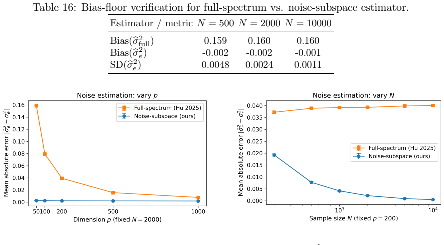
C.5 PPCA noise variance verification The spectral estimator coincides with the PPCA noise MLE in the single-view setting

0.098801 0.001450 Tipping & Bishop MLE 0.098801 0.001450 MSE, while both methods are comparable on Σ t, consistent with EM being tightly matched to the specialized model. C.5 PPCA noise variance verification The spectral estimator coincides with the PPCA noise MLE in the single-view setting. C.6 Numerical confirmation of the Hu-bias floor Table 16 confirm...

work page 2000
[16]

inverse normal transform (Rank-INT)

suffers from a O(r/p) bias floor, while the noise-subspace estimator (ours) is essentially unbiased. inverse normal transform (Rank-INT). Table 18 reports prediction MSE and calibration coverage at nominal levels 95%, 90%, and 80%. The ’Gaussian (ref)’ row uses the Gaussian benchmark from Section 6.3.2 under the same nominal high-noise tuple; it serves as...

work page 2000