arxiv: 2605.12768 · v1 · submitted 2026-05-12 · 📊 stat.ML · cs.LG

Recognition: no theorem link

ISOMORPH: A Supply Chain Digital Twin for Simulation, Dataset Generation, and Forecasting Benchmarks

Zhizhen Zhang , Hyemin Gu , Benjamin J. Zhang , Daniel Elenius , Michael Tyrrell , Theo J. Bourdais , Houman Owhadi , Markos A. Katsoulakis

show 1 more author

Tuhin Sahai

Authors on Pith no claims yet

Pith reviewed 2026-05-14 19:27 UTC · model grok-4.3

classification 📊 stat.ML cs.LG

keywords supply chaindigital twintime series forecastingfoundation modelsbullwhip effectbenchmarkuncertainty quantificationsimulation

0 comments

The pith

ISOMORPH creates the first public digital twin of a multi-echelon supply chain to generate forecasting benchmarks and test foundation models.

A machine-rendered reading of the paper's core claim, the machinery that carries it, and where it could break.

This paper presents ISOMORPH, a simulator that models a logistics network as a directed graph advancing in discrete time steps. Demand arrives and is fulfilled from stock or backlogged, with replenishments propagating through the network according to configurable rules. The state evolves as a Markov chain on inventory levels, orders, and demand estimates, naturally producing the bullwhip effect in released datasets. Foundation models evaluated zero-shot on this data achieve better MASE scores than on standard benchmarks at short horizons, and parameter perturbations generate confidence intervals showing the models can approximate uncertainty from the full simulator. Supply chain forecasting has lacked such open, interpretable testbeds, so this enables direct comparison and extension of existing time-series methods to logistics problems.

Core claim

The central discovery is a fully interpretable digital twin simulator for multi-echelon supply chains that advances a routing graph in discrete time, tracks a Markovian state vector of inventories and flows, and reproduces empirically consistent bullwhip dynamics. Released datasets from two catalogue sizes with scenario sweeps and Latin-hypercube perturbations exhibit variance amplification, bottlenecks, and cross-channel effects. Zero-shot tests on four foundation models yield MASE values exceeding GIFT-Eval references at low-to-moderate horizons, and the same setup produces forecast bands via demand knob perturbations, establishing foundation models as fast surrogates for the twin'sforward

What carries the argument

The Markov chain transition kernel on the state vector of per-node on-hand inventory, outstanding orders, in-transit shipments, and smoothed demand estimate, which linearly acts on the empirical distribution and closes the dynamics while encoding conservation laws.

Load-bearing premise

The discrete-time rules and state transitions in the simulator produce dynamics that match real supply-chain phenomena like the bullwhip effect at consistent magnitudes, even without calibration to proprietary data.

What would settle it

Observing that the generated rollouts do not exhibit variance amplification matching empirical bullwhip magnitudes, or that foundation model MASE scores fall below GIFT-Eval references under identical evaluation protocols.

Figures

Figures reproduced from arXiv: 2605.12768 by Benjamin J. Zhang, Daniel Elenius, Houman Owhadi, Hyemin Gu, Markos A. Katsoulakis, Michael Tyrrell, Theo J. Bourdais, Tuhin Sahai, Zhizhen Zhang.

**Figure 1.** Figure 1: The ISOMORPH model. (a) Released network: 13 U.S. cities (3 sources, 9 intermediate warehouses across 5 tiers, and destination NewYork) connected by 16 directed edges, each carrying a user-set transit time τe; the map shows geographic placement, but the graph structure and routing are defined by the edges and their transit times, not by geographic distance. (b) Dynamic Bayesian network across three time sl… view at source ↗

**Figure 2.** Figure 2: One-step transition map Ψ : ξt 7→ ξt+1 as a fixed sequence of seven sub-steps (Algorithm 1). Random external inputs (violet, top) enter at exactly two sub-steps—demand yt at sub-step (4) and source lead times Lt at sub-step (7); the remaining five sub-steps are deterministic bookkeeping given (ξt, yt, Lt). Sub-steps (1) and (2) integrate inbound arrivals due at t, (3) replenishes per-step edge capacity, (4… view at source ↗

**Figure 3.** Figure 3: The ISOMORPH model as a dynamic Bayesian network across three time slices. Random external inputs (top row, violet): demand yt ∼ Poisson(λi,t) and source lead times Lt are the only sources of randomness in the chain. The intensity λ (orange) is deterministic given the simulator seed. Markov state (bottom row, dashed boxes): the state ξt is the joint state of the simulator, transitioned by the deterministic… view at source ↗

**Figure 4.** Figure 4: Diversity of dynamics generated by the simulator for a single item (I36) across four [PITH_FULL_IMAGE:figures/full_fig_p020_4.png] view at source ↗

**Figure 5.** Figure 5: Forward UQ forecast envelope for item I01 at one forecast window. Each panel shows a [PITH_FULL_IMAGE:figures/full_fig_p023_5.png] view at source ↗

**Figure 6.** Figure 6: Baseline release at C=50, raw values at each time unit. Left column (a, c, e): for items I01– I03 over the full T=52,560 time units horizon, the daily demand (blue), the part served immediately from inventory at the destination (amber), and the part left unmet (red, shaded). Per-item fill rates appear in each panel’s title; the yellow band marks the zoom window shown on the right. Right column (b, d, f): t… view at source ↗

**Figure 7.** Figure 7: Forward UQ forecast envelopes for item I01 at three forecast windows ( [PITH_FULL_IMAGE:figures/full_fig_p035_7.png] view at source ↗

read the original abstract

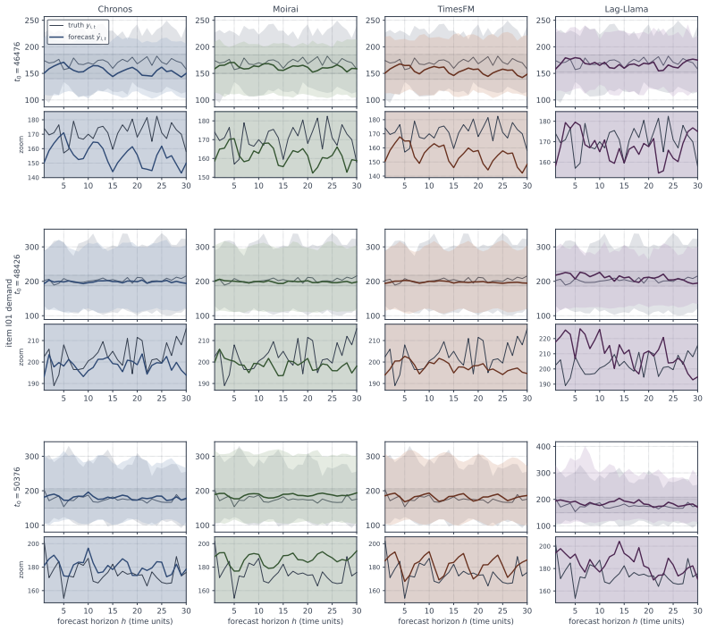
Open time-series forecasting (TSF) benchmarks cover retail, energy, weather, and traffic, but supply-chain logistics remains underserved. We introduce ISOMORPH, the first public digital twin of a multi-echelon logistics network with fully interpretable, user-configurable parameters and modular topology, demand process, and control rules. The simulator advances a directed routing graph in discrete time: demand arrives at the destination, is served from stock or recorded as backlog, and triggers replenishment through the network. The state vector tracks per-node on-hand inventory with outstanding orders, in-transit shipments, and a smoothed demand estimate, so the dynamics close as a Markov chain on a tractable state space whose transition kernel acts linearly on the empirical distribution of the state. The released data reproduces the bullwhip effect at empirically consistent magnitudes, and three conservation laws encoded in the Markov chain serve as verification tools when users extend the simulator. We release datasets at two catalogue scales ($C=50$ and $C=200$) with six scenario sweeps producing 30 additional rollouts and 20 Latin-hypercube perturbations, exhibiting dynamics absent from fixed TSF benchmarks: variance amplification, cascading bottlenecks, regime shifts, and cross-channel coupling through shared macro shocks. Zero-shot evaluation of four foundation models (Chronos, Moirai, TimesFM, Lag-Llama) shows MASE values exceeding public GIFT-Eval references at low-to-moderate horizons, supporting incorporation into existing benchmarks. The same pairing produces forecast confidence bands via Latin-hypercube perturbation of demand-side knobs, forward UQ from parameter uncertainty unavailable on standard TSF datasets, demonstrating that foundation models can serve as fast surrogates for the digital twin's forward UQ. Code (MIT): https://github.com/tuhinsahai/ISOMORPH.

Editorial analysis

A structured set of objections, weighed in public.

Desk editor's note, referee report, simulated authors' rebuttal, and a circularity audit. Tearing a paper down is the easy half of reading it; the pith above is the substance, this is the friction.

Desk Editor's Note private letter to a colleague

ISOMORPH delivers a practical open simulator and datasets for supply-chain forecasting that capture network effects missing from standard benchmarks, but its dynamics rest on uncalibrated rules.

read the letter

ISOMORPH is worth knowing about because it gives the community an open, configurable simulator for generating supply chain time series that include realistic network interactions like the bullwhip effect. They model a multi-echelon logistics network in discrete time. Demand hits the end nodes, gets filled from stock or backlogged, and triggers replenishments upstream. The state keeps track of on-hand inventory, outstanding orders, in-transit items, and a smoothed demand signal. This setup forms a Markov chain whose transition acts linearly on the state distribution. Three conservation laws are built in for verification when users change the rules. The released datasets cover two catalogue sizes and include scenario sweeps plus Latin-hypercube perturbations of demand parameters. These trajectories show variance amplification, cascading bottlenecks, regime shifts, and coupling across channels. Zero-shot tests on Chronos, Moirai, TimesFM, and Lag-Llama yield MASE values that exceed some GIFT-Eval baselines at shorter horizons. The same setup produces forecast intervals by perturbing the knobs, which is a clean way to get uncertainty from the digital twin. The soft spot is validation against reality. The paper states that the data reproduces the bullwhip effect at empirically consistent magnitudes, yet the description relies entirely on the user-set parameters and discrete rules without any quantitative comparison to real operational traces or published amplification statistics from industry. Internal checks pass, but that does not confirm the magnitudes match what happens in actual supply chains. This work is for forecasting researchers who want benchmarks that go beyond standard retail or energy series and include explicit uncertainty sources. Anyone evaluating foundation models or building surrogates for logistics simulation will find the code and data directly usable. It has enough new artifacts and addresses a documented gap, so it should receive a serious referee. I recommend sending it to peer review.

Referee Report

2 major / 2 minor

Summary. The paper introduces ISOMORPH, a configurable digital twin simulator for multi-echelon supply-chain networks that advances a directed routing graph in discrete time, maintains a Markov-closed state vector of inventory, orders, and demand estimates, and releases synthetic datasets at catalogue scales C=50 and C=200. These datasets exhibit variance amplification, cascading bottlenecks, and regime shifts; the authors report that they reproduce the bullwhip effect at empirically consistent magnitudes. Zero-shot evaluations of four foundation models (Chronos, Moirai, TimesFM, Lag-Llama) yield MASE values exceeding public GIFT-Eval references at low-to-moderate horizons, and Latin-hypercube perturbations of demand parameters are used to generate forecast confidence bands, positioning the simulator as a source of forward UQ unavailable in standard TSF benchmarks.

Significance. If the simulator's discrete-time rules and conservation-law checks produce trajectories whose statistical properties align with real multi-echelon logistics, ISOMORPH would fill a documented gap in open TSF benchmarks by supplying interpretable, user-extensible data together with built-in verification. The foundation-model MASE results and surrogate-UQ demonstration would then provide a concrete basis for incorporating supply-chain scenarios into existing evaluation suites.

major comments (2)

[Abstract / Simulator description] Abstract and simulator section: the claim that the released data 'reproduces the bullwhip effect at empirically consistent magnitudes' is not accompanied by quantitative comparisons (e.g., order-variance amplification ratios) against published retail or manufacturing studies; verification is restricted to three conservation laws and synthetic rollouts, leaving open whether the observed dynamics contain artifacts of the linear transition kernel or the chosen demand process.
[Forecasting experiments] Forecasting experiments: the statement that foundation-model MASE values exceed GIFT-Eval references at low-to-moderate horizons lacks tabulated per-horizon scores, number of independent rollouts, and confidence intervals, so the robustness of the 'supporting incorporation' conclusion cannot be assessed from the reported results.

minor comments (2)

The GitHub repository link is given, but the manuscript should specify the exact parameter files or seeds used to generate the two released catalogue-scale datasets so that users can exactly reproduce the published rollouts.
[Simulator description] Notation for the state vector components (on-hand inventory, outstanding orders, in-transit shipments, smoothed demand) should be introduced once in a single table or equation block rather than scattered across the simulator description.

Simulated Author's Rebuttal

2 responses · 0 unresolved

We thank the referee for their thoughtful comments on our manuscript. We address each major comment below and outline the revisions we will implement to improve clarity and completeness.

read point-by-point responses

Referee: [Abstract / Simulator description] Abstract and simulator section: the claim that the released data 'reproduces the bullwhip effect at empirically consistent magnitudes' is not accompanied by quantitative comparisons (e.g., order-variance amplification ratios) against published retail or manufacturing studies; verification is restricted to three conservation laws and synthetic rollouts, leaving open whether the observed dynamics contain artifacts of the linear transition kernel or the chosen demand process.

Authors: We agree that providing quantitative comparisons to published empirical studies would better support the claim of reproducing the bullwhip effect at consistent magnitudes. In the revised version, we will add a dedicated subsection or table that computes and reports order-variance amplification ratios from the ISOMORPH datasets and directly compares them to values from key literature (such as studies on retail and manufacturing supply chains). We will also elaborate on the design choices for the linear transition kernel and demand process to mitigate concerns about artifacts, including additional verification through sensitivity analyses on parameter perturbations. revision: yes
Referee: [Forecasting experiments] Forecasting experiments: the statement that foundation-model MASE values exceed GIFT-Eval references at low-to-moderate horizons lacks tabulated per-horizon scores, number of independent rollouts, and confidence intervals, so the robustness of the 'supporting incorporation' conclusion cannot be assessed from the reported results.

Authors: We acknowledge the need for more detailed reporting to allow assessment of robustness. In the revision, we will include tabulated per-horizon MASE scores for each foundation model, explicitly state the number of independent rollouts used (noting the 30 scenario sweeps and additional perturbations mentioned), and provide confidence intervals or standard deviations for the metrics. This will strengthen the evidence for incorporating supply-chain scenarios into TSF benchmarks. revision: yes

Circularity Check

0 steps flagged

No significant circularity; simulator rules and evaluations are self-contained

full rationale

The paper defines the ISOMORPH simulator explicitly via user-configurable routing graph, discrete-time inventory/backlog/replenishment rules, and a state vector whose Markov transition kernel is derived directly from those rules. Conservation laws act as independent verification checks rather than fitted targets. Datasets are produced by forward simulation, foundation-model MASE evaluations and Latin-hypercube UQ bands are computed on the generated trajectories, and the bullwhip reproduction claim follows from the chosen rule magnitudes without any reduction to a self-fit or self-citation by construction. All load-bearing steps remain independent of the claimed outputs.

Axiom & Free-Parameter Ledger

1 free parameters · 1 axioms · 0 invented entities

The central claim rests on the assumption that the chosen state vector renders the supply-chain dynamics Markovian and that the conservation laws hold exactly; no new physical entities are postulated and no parameters are fitted to external data for the reported results.

free parameters (1)

catalogue scale C
User-configurable network size set to 50 and 200 for released datasets; not fitted to observed data.

axioms (1)

domain assumption The state vector (on-hand inventory, outstanding orders, in-transit shipments, smoothed demand) renders the network dynamics a Markov chain whose transition kernel acts linearly on the empirical state distribution.
Invoked to close the dynamics and enable verification via conservation laws.

pith-pipeline@v0.9.0 · 5678 in / 1440 out tokens · 64677 ms · 2026-05-14T19:27:59.066766+00:00 · methodology

discussion (0)

Reference graph

Works this paper leans on

12 extracted references · 9 canonical work pages · 1 internal anchor

[1]

Deepbullwhip: An Open-Source Simulation and Benchmarking for Multi-Echelon Bullwhip Analyses

doi: 10.48550/arXiv.2604.13478. Tom Beucler, Michael Pritchard, Stephan Rasp, Jordan Ott, Pierre Baldi, and Pierre Gentine. Enforc- ing analytic constraints in neural networks emulating physical systems.Physical Review Letters, 126(9):098302,

work page internal anchor Pith review Pith/arXiv arXiv doi:10.48550/arxiv.2604.13478
[2]

Gérard Cachon, Taylor Randall, and Glen Schmidt

doi: 10.1103/PhysRevLett.126.098302. Gérard Cachon, Taylor Randall, and Glen Schmidt. In search of the bullwhip effect.Manufacturing & Service Operations Management, 9:457–479, 10

work page doi:10.1103/physrevlett.126.098302
[3]

Hong Chen and David D

doi: 10.1287/msom.1060.0149. Hong Chen and David D. Yao.Fundamentals of Queueing Networks: Performance, Asymptotics, and Optimization. Stochastic Modelling and Applied Probability. Springer,

work page doi:10.1287/msom.1060.0149
[4]

24 Christian D

URL https: //openreview.net/forum?id=wEc1mgAjU-. 24 Christian D. Hubbs, Hector D. Perez, Owais Sarwar, Nikolaos V . Sahinidis, Ignacio E. Grossmann, and John M. Wassick. Or-gym: A reinforcement learning library for operations research problem.ArXiv, abs/2008.06319,

work page arXiv 2008
[5]

Spyros Makridakis, Evangelos Spiliotis, and Vassilios Assimakopoulos

doi: 10.1016/j.ijforecast.2019.04.014. Spyros Makridakis, Evangelos Spiliotis, and Vassilios Assimakopoulos. M5 accuracy competition: Results, findings, and conclusions.International Journal of Forecasting, 38(4):1346–1364,

work page doi:10.1016/j.ijforecast.2019.04.014 2019
[6]

Azmine Toushik Wasi, MD Shafikul Islam, and Adipto Raihan Akib

doi: 10.1016/j.jcp.2021.110551. Azmine Toushik Wasi, MD Shafikul Islam, and Adipto Raihan Akib. Supplygraph: A benchmark dataset for supply chain planning using graph neural networks.ArXiv, abs/2401.15299,

work page doi:10.1016/j.jcp.2021.110551 2021
[7]

Ward Whitt.Stochastic-Process Limits: An Introduction to Stochastic-Process Limits and Their Application to Queues

doi: 10.1029/2021MS002954. Ward Whitt.Stochastic-Process Limits: An Introduction to Stochastic-Process Limits and Their Application to Queues. Springer Series in Operations Research. Springer,

work page doi:10.1029/2021ms002954
[8]

CoRR abs/2012.07436 (2020)

doi: 10.48550/arXiv.2012.07436. 25 A Parameter values This appendix lists the parameter values used to produce the released runs. The algorithms that use these parameters are in §3.3. A.1 Demand-generator coefficients Each item i draws its demand-process coefficients independently from the distributions of Table

work page doi:10.48550/arxiv.2012.07436 2012
[9]

Key” is the combination of columns that uniquely identifies a row. “Rows

All values are the script’s built-in defaults, except for the pipeline multiplierm. The default m= 0 selects a reactive shipping rule that ships against backlog plus a three-time-unit buffer of smoothed demand; m= 7 selects the proactive rule used in this work, which keeps seven time units of smoothed demand in the pipeline at all times. 27 Table 8: Runti...

2025
[10]

Table 13 lists all six sweeps; the baseline value is bold in each row

To study how the network’s behavior and the resulting time series change under different operating conditions, we construct six one-at-a-time sweeps: each varies a single knob across five settings—a shared baseline (all knobs at default) plus four perturbations—while holding all other knobs at baseline, producing 6×5 = 30rollouts on theC=50regime. Table 1...

work page arXiv
[11]

Model baseline shock_xhi drift_mid chaos_comp

Best per column within eachh-block inbold. Model baseline shock_xhi drift_mid chaos_comp. burst_xhi chaos_burst h=1 Chronos 0.769 0.779 0.761 0.768 0.638 0.643 Moirai 0.786 0.805 0.785 0.795 0.663 0.678 TimesFM0.742 0.748 0.737 0.743 0.628 0.638 Lag-Llama 1.027 1.080 1.014 1.070 1.059 1.085 h=7 Chronos 0.818 0.822 0.798 0.817 0.7880.781 Moirai 0.831 0.845...

2048
[12]

The wide spread between Baltimore and Philadelphia in the daily column reflects sub-monthly batching of arrivals, which the monthly column smooths out. Node Tier Daily ¯Bn Monthly ¯Bn NewYork Destination9.03 1.43 Baltimore Tier-56.83 1.64 Philadelphia Tier-519.16 1.49 Columbus Tier-41.39 1.27 Richmond Tier-41.40 1.34 Charlotte Tier-31.15 1.33 Chicago Tier...

2080