arxiv: 2605.13671 · v1 · submitted 2026-05-13 · 🧮 math-ph · cs.NA· math.MP· math.NA· math.PR· physics.flu-dyn

Recognition: unknown

Stochastic modeling of Fourier modes in two-dimensional turbulence via filtered white noise

Paolo Cifani , Franco Flandoli , Andrea Zanoni

Authors on Pith no claims yet

Pith reviewed 2026-05-14 17:47 UTC · model grok-4.3

classification 🧮 math-ph cs.NAmath.MPmath.NAmath.PRphysics.flu-dyn

keywords stochastic modelingFourier modestwo-dimensional turbulencepassive tracereffective diffusionfiltered white noisedirect numerical simulation

0 comments

The pith

A stochastic model of Fourier modes driven by filtered white noise reproduces the effective diffusion of passive tracers in two-dimensional turbulence.

A machine-rendered reading of the paper's core claim, the machinery that carries it, and where it could break.

The paper examines the time series of Fourier modes in forced two-dimensional turbulence and identifies a characteristic correlation time. It then constructs a simple stochastic model in which each mode evolves as an independent process driven by filtered white noise. Direct numerical simulations of the turbulent flow and of the stochastic model are used to compute the transport of a passive tracer. The effective diffusion coefficients obtained from the two approaches agree closely. This suggests that the reduced stochastic description captures the essential statistics governing convective transport without requiring the full nonlinear dynamics.

Core claim

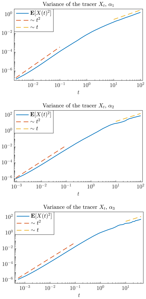
The authors propose modeling the Fourier components of the velocity field in two-dimensional turbulence as independent Ornstein-Uhlenbeck-like processes driven by filtered white noise, with a single correlation length chosen to match the observed time correlations. When this model is substituted into the advection equation for a passive scalar, the resulting mean-square displacement and effective diffusivity match those computed from full direct numerical simulations of the Navier-Stokes equations.

What carries the argument

The stochastic model for Fourier modes, where each mode is driven by filtered white noise with a fitted correlation time.

Load-bearing premise

That the Fourier modes behave as independent processes whose individual time correlations fully determine the transport statistics, without significant contributions from nonlinear cross-mode interactions.

What would settle it

Running the stochastic model with the same correlation length but observing a mismatch in the tracer's mean-square displacement beyond statistical error bars in a new simulation at higher Reynolds number.

Figures

Figures reproduced from arXiv: 2605.13671 by Andrea Zanoni, Franco Flandoli, Paolo Cifani.

**Figure 1.** Figure 1: Vorticity field ω and energy spectrum Ek at the final time step of the simulation, for decreasing values of the damping parameter α, i.e., α1 > α2 > α3 > 0. 3 [PITH_FULL_IMAGE:figures/full_fig_p003_1.png] view at source ↗

**Figure 2.** Figure 2: Trajectories of several Fourier modes with forcing applied at [PITH_FULL_IMAGE:figures/full_fig_p006_2.png] view at source ↗

**Figure 3.** Figure 3: Trajectories of several Fourier modes with forcing applied at [PITH_FULL_IMAGE:figures/full_fig_p007_3.png] view at source ↗

**Figure 4.** Figure 4: Distribution of several Fourier modes with forcing applied at [PITH_FULL_IMAGE:figures/full_fig_p007_4.png] view at source ↗

**Figure 5.** Figure 5: Distribution of several Fourier modes with forcing applied at [PITH_FULL_IMAGE:figures/full_fig_p008_5.png] view at source ↗

**Figure 6.** Figure 6: Heatmap of the absolute value of the correlations between different [PITH_FULL_IMAGE:figures/full_fig_p009_6.png] view at source ↗

**Figure 7.** Figure 7: Estimated relaxation time τk for different Fourier modes, with forcing applied at |k| ∼ kf = 50 (left) and |k| ∼ kf = 100 (right). where the coefficient 2 is justified in Section 5. The autocorrelation function Rk(∆) is estimated from the data by temporal averages using the MATLAB function autocorr (Econometrics Toolbox), which provides a standard and numerically stable implementation. The estimated relax… view at source ↗

**Figure 8.** Figure 8: Autocorrelation function Rk(∆) rescaled by the relaxation time τk and normalized variance of the increments Vk(∆) for different Fourier modes, with forcing applied at |k| ∼ kf = 50. This can be explained by the fact that, although we construct stochastic models, the underlying partial differential equation and the numerical simulations are deterministic except for the forcing term. As a result, the Fourier… view at source ↗

**Figure 9.** Figure 9: Autocorrelation function Rk(∆) rescaled by the relaxation time τk and normalized variance of the increments Vk(∆) for different Fourier modes, with forcing applied at |k| ∼ kf = 100. of samples from the trajectory. Then, an approximate confidence interval with confidence level ℓ for Rk(nδ), n = 1, . . . , N, is Rk(nδ) ± z 1+ℓ 2 vuuut 1 N  1 + 2 nX−1 j=1 Rk(jδ) 2  , (11) where z 1+ℓ 2 is the quantile of… view at source ↗

**Figure 10.** Figure 10: Approximate 95% confidence intervals for the autocorrelation func [PITH_FULL_IMAGE:figures/full_fig_p012_10.png] view at source ↗

**Figure 11.** Figure 11: Approximate 95% confidence intervals for the autocorrelation func [PITH_FULL_IMAGE:figures/full_fig_p012_11.png] view at source ↗

**Figure 12.** Figure 12: Simulated trajectories of the model for different values of [PITH_FULL_IMAGE:figures/full_fig_p017_12.png] view at source ↗

**Figure 13.** Figure 13: Autocorrelation function Cβ from theorem 5 and the function 2(1 − Cβ), corresponding to the statistics in equations (8) and (9) for the vorticity field, respectively, for different values of the parameter β. 18 [PITH_FULL_IMAGE:figures/full_fig_p018_13.png] view at source ↗

**Figure 14.** Figure 14: Autocorrelation function Rk(∆) and normalized variance of the increments Vk(∆), both rescaled by the relaxation time τk, for different Fourier modes with forcing applied at |k| ∼ kf = 50, compared with the Gaussian kernel model. to theorems 3 and 4, we expect Rk(∆) ≃ C ∆ τk , Vk(∆) ≃ 1 − C ∆ τk , which is confirmed numerically. The model shows strong agreement with the data for most Fourier modes… view at source ↗

**Figure 15.** Figure 15: Autocorrelation function Rk(∆) and normalized variance of the increments Vk(∆), both rescaled by the relaxation time τk, for different Fourier modes with forcing applied at |k| ∼ kf = 100, compared with the Gaussian kernel model. 4 The velocity field We now have all the ingredients needed to construct a stochastic model for the velocity field based on (4). For the temporal processes ξ k t , we adopt the … view at source ↗

**Figure 16.** Figure 16: Variance of the tracer Xt, for decreasing values of the damping parameter α, i.e., α1 > α2 > α3 > 0. 26 [PITH_FULL_IMAGE:figures/full_fig_p026_16.png] view at source ↗

read the original abstract

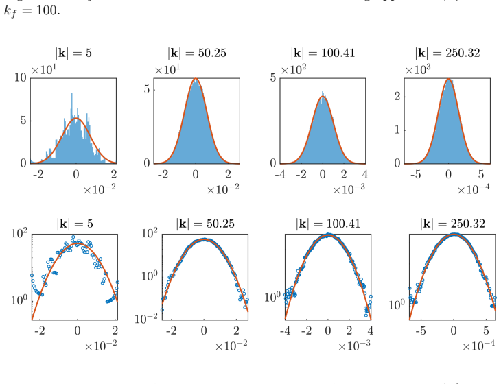
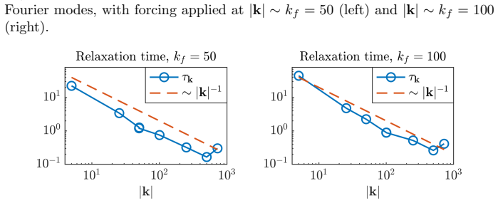
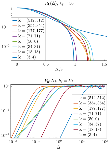
Modeling turbulent flows by a random Fourier decomposition is a classical procedure in order to use simplified models of turbulence in heat transport and other applications. We carefully investigate the Fourier time series of two-dimensional turbulent flows forced at intermediate scales and identify significant statistical structures. In particular, we find the existence of a typical time correlation length, and propose a stochastic model for the Fourier components. Finally, we compute the transport of a passive tracer under purely convective dynamics by means of direct numerical simulation of the turbulent flow and compare it with the effective diffusion produced by the stochastic model.

Editorial analysis

A structured set of objections, weighed in public.

Desk editor's note, referee report, simulated authors' rebuttal, and a circularity audit. Tearing a paper down is the easy half of reading it; the pith above is the substance, this is the friction.

Desk Editor's Note private letter to a colleague

The paper builds a filtered-white-noise model for independent Fourier modes in 2D turbulence matched to a single correlation time and checks the resulting tracer diffusivity against DNS, but the match is stated without numbers or robustness checks.

read the letter

The core move is to extract a typical time correlation length from the Fourier time series of forced 2D turbulence, then drive each mode with filtered white noise using that length, and finally compare the long-time diffusion of a passive tracer under the reconstructed velocity field to the same quantity from full DNS. That end-to-end construction is the concrete piece that is new here. It gives a reduced-order way to generate velocity fields that preserve at least the single-time-scale statistics while remaining cheap enough for transport calculations. The authors also run the tracer advection in both the stochastic and the direct cases, which is the right test for the intended use in heat-transport modeling. That part is done cleanly enough on paper. The soft spots are in the evidence. The abstract reports that a comparison was performed but supplies no diffusivity values, no error estimates, and no description of how the filter cutoff or correlation length was chosen or cross-validated. Because the length is measured on the same runs later used for the transport test, any agreement could be partly by construction. The independence assumption across modes is another open question; the Navier-Stokes nonlinearity produces cross-spectra and phase relations that the model drops, and it is not obvious that these are negligible for integrated advection. A reader working on reduced turbulence models or scalar transport would find the construction useful to know about and could test it themselves on their own flows. The work is coherent on its own terms and shows clear thinking about what statistics to keep, so it deserves a serious referee rather than a desk rejection. I would send it out.

Referee Report

3 major / 2 minor

Summary. The paper examines Fourier time series from two-dimensional turbulence forced at intermediate scales, identifies a characteristic time correlation length, and constructs a stochastic model in which each Fourier mode evolves as an independent process driven by filtered white noise. It then computes the long-time effective diffusivity of a passive tracer advected by the reconstructed velocity field and compares this diffusivity with the value obtained from direct numerical simulation of the full Navier-Stokes equations.

Significance. If the reported agreement in effective diffusivity is confirmed by quantitative metrics, the approach would supply a low-dimensional stochastic surrogate for turbulent advection that avoids resolving nonlinear mode coupling, offering a practical simplification for transport calculations in two-dimensional flows.

major comments (3)

[Abstract] Abstract: the claim that the stochastic model reproduces the DNS effective diffusivity is stated without any quantitative measure (error bars, relative error, or statistical test), without specification of how the filter parameters were selected, and without description of the Reynolds-number or forcing-scale range tested. This absence leaves the central claim unsupported by visible evidence.
[Model construction and validation sections] Model construction and validation sections: the single correlation length used to define the filter is extracted from the identical DNS runs whose tracer statistics are later compared to the model output. This procedure renders the comparison circular; the model is tuned to the very data it is asked to reproduce.
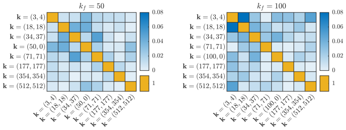
[Independence assumption for Fourier modes] Independence assumption for Fourier modes: the model treats modes as statistically independent, yet the Navier-Stokes nonlinearity generates non-zero cross-spectra and phase correlations that contribute to coherent structures and integrated advection. The manuscript provides no test showing that these omitted correlations are negligible for the long-time tracer dispersion.

minor comments (2)

[Notation and filter definition] Clarify the precise functional form of the filter applied to the white-noise forcing and the numerical procedure used to extract the correlation length from the time series.
[Results] Add a brief discussion of the Reynolds-number dependence of the reported correlation length to indicate the regime of validity.

Simulated Author's Rebuttal

3 responses · 0 unresolved

We thank the referee for the insightful comments on our manuscript arXiv:2605.13671. We address each of the major comments below and outline the revisions we plan to make.

read point-by-point responses

Referee: [Abstract] Abstract: the claim that the stochastic model reproduces the DNS effective diffusivity is stated without any quantitative measure (error bars, relative error, or statistical test), without specification of how the filter parameters were selected, and without description of the Reynolds-number or forcing-scale range tested. This absence leaves the central claim unsupported by visible evidence.

Authors: We agree with the referee that the abstract should include quantitative measures to support the claim. In the revised manuscript, we will add the relative error between the effective diffusivities from the stochastic model and DNS, along with standard deviations from ensemble runs. We will also specify the method for selecting filter parameters and the tested ranges of Reynolds numbers and forcing scales. revision: yes
Referee: [Model construction and validation sections] Model construction and validation sections: the single correlation length used to define the filter is extracted from the identical DNS runs whose tracer statistics are later compared to the model output. This procedure renders the comparison circular; the model is tuned to the very data it is asked to reproduce.

Authors: The referee is correct that the correlation length is determined from the same DNS simulations used for the tracer comparison, which introduces a degree of circularity. We will revise the manuscript to explicitly state this and discuss the implications. Additionally, we will include a sensitivity analysis showing how the effective diffusivity depends on the choice of correlation length, and consider using correlation lengths from independent runs or theoretical predictions in future extensions. revision: yes
Referee: [Independence assumption for Fourier modes] Independence assumption for Fourier modes: the model treats modes as statistically independent, yet the Navier-Stokes nonlinearity generates non-zero cross-spectra and phase correlations that contribute to coherent structures and integrated advection. The manuscript provides no test showing that these omitted correlations are negligible for the long-time tracer dispersion.

Authors: We recognize that assuming statistical independence of Fourier modes neglects cross-correlations arising from nonlinear interactions. The manuscript does not provide a direct test of their impact on tracer dispersion. In the revision, we will add a section comparing the power spectrum and velocity correlations with and without the independence assumption, and perform additional numerical experiments to quantify the effect on long-time effective diffusivity. revision: yes

Circularity Check

1 steps flagged

Correlation length fitted from DNS Fourier time series then used to drive stochastic model whose tracer diffusivity is compared to the same DNS

specific steps

fitted input called prediction [Abstract (model construction and comparison paragraph)]
"we find the existence of a typical time correlation length, and propose a stochastic model for the Fourier components. Finally, we compute the transport of a passive tracer under purely convective dynamics by means of direct numerical simulation of the turbulent flow and compare it with the effective diffusion produced by the stochastic model."

The correlation length is measured on the DNS velocity field; that measured length is then used to define the stochastic forcing of the model; the model's output diffusivity is finally compared to the diffusivity measured on the same DNS. The match is therefore a test of whether the model, once its single parameter has been set to the data, reproduces a statistic derived from the same data.

full rationale

The paper extracts a typical time correlation length directly from the Fourier time series of the forced 2D turbulence DNS. This single length is inserted into the filtered-white-noise driving term of the independent-mode stochastic model. The model is then integrated to produce an effective diffusivity for a passive tracer, which is compared to the diffusivity obtained from the original DNS. Because the sole free parameter of the stochastic model is taken from the identical data set whose transport statistics are later reproduced, the reported agreement reduces to a consistency check on the fitted input rather than an independent derivation or out-of-sample prediction.

Axiom & Free-Parameter Ledger

1 free parameters · 1 axioms · 0 invented entities

The approach rests on extracting a single correlation length from simulation data and assuming that independent filtered-white-noise processes for each mode suffice to reproduce integrated transport statistics.

free parameters (1)

time correlation length
Measured from the Fourier time series and used to define the filter applied to white noise.

axioms (1)

domain assumption Fourier modes evolve independently
The stochastic model treats each mode as an independent process.

pith-pipeline@v0.9.0 · 5402 in / 1176 out tokens · 53878 ms · 2026-05-14T17:47:15.530688+00:00 · methodology

discussion (0)

Reference graph

Works this paper leans on

37 extracted references · 1 canonical work pages

[1]

Apolin´ ario, Geoffrey Beck, Laurent Chevillard, Isabelle Gal- lagher, and Ricardo Grande

Gabriel B. Apolin´ ario, Geoffrey Beck, Laurent Chevillard, Isabelle Gal- lagher, and Ricardo Grande. A linear stochastic model of turbulent cas- cades and fractional fields.Ann. Sc. Norm. Super. Pisa Cl. Sci. (5), 26(4):2043–2103, 2025

2043
[2]

Apolin´ ario, Laurent Chevillard, and Jean-Christophe Mourrat

Gabriel B. Apolin´ ario, Laurent Chevillard, and Jean-Christophe Mourrat. Dynamical fractional and multifractal fields.J. Stat. Phys., 186(1):Paper No. 15, 35, 2022

2022
[3]

Stochastic model reduction: convergence and applications to climate equations.J

Sigurd Assing, Franco Flandoli, and Umberto Pappalettera. Stochastic model reduction: convergence and applications to climate equations.J. Evol. Equ., 21(4):3813–3848, 2021

2021
[4]

Boffetta and S

G. Boffetta and S. Musacchio. Evidence for the double cascade scenario in two-dimensional turbulence.Phys. Rev. E, 82:016307, Jul 2010

2010
[5]

Guido Boffetta and Robert E. Ecke. Two-dimensional turbulence. InAn- nual review of fluid mechanics. Volume 44, 2012, volume 44 ofAnnu. Rev. Fluid Mech., pages 427–451. Annual Reviews, Palo Alto, CA, 2012

2012
[6]

George E. P. Box and Gwilym M. Jenkins.Time series analysis: forecasting and control. Holden-Day Series in Time Series Analysis. Holden-Day, San Francisco, Calif.-D¨ usseldorf-Johannesburg, revised edition, 1976

1976
[7]

Canuto, M

C. Canuto, M. Y. Hussaini, A. Quarteroni, and T. A. Zang.Spectral meth- ods. Scientific Computation. Springer, Berlin, 2007. Evolution to complex geometries and applications to fluid dynamics

2007
[8]

Springer, Cham, [2023]©2023

Bertrand Chapron, Dan Crisan, Darryl Holm, Etienne M´ emin, and Anna Radomska, editors.Stochastic transport in upper ocean dynamics, vol- ume 10 ofMathematics of Planet Earth. Springer, Cham, [2023]©2023. STUOD 2021 Workshop, London, UK, September 20–23

2023
[9]

Laurent Chevillard, Marc Lagoin, and Stephane G. Roux. Multifractal fractional ornstein-uhlenbeck processes. Preprint arXiv:2011.09503, 2021

work page arXiv 2011
[10]

Diffusion properties of small-scale frac- tional transport models.J

Paolo Cifani and Franco Flandoli. Diffusion properties of small-scale frac- tional transport models.J. Stat. Phys., 192(11):Paper No. 152, 20, 2025

2025
[11]

Variational principles for fully coupled stochastic fluid dynamics across scales.Phys

Arnaud Debussche and Etienne M´ emin. Variational principles for fully coupled stochastic fluid dynamics across scales.Phys. D, 481:Paper No. 134777, 11, 2025

2025
[12]

Second order perturbation theory of two-scale systems in fluid dynamics.J

Arnaud Debussche and Umberto Pappalettera. Second order perturbation theory of two-scale systems in fluid dynamics.J. Eur. Math. Soc. (JEMS), 28(4):1533–1595, 2026. 28

2026
[13]

Ephrati, Paolo Cifani, Erwin Luesink, and Bernard J

Sagy R. Ephrati, Paolo Cifani, Erwin Luesink, and Bernard J. Geurts. Data-driven stochastic Lie transport modeling of the 2D euler equations. Journal of Advances in Modeling Earth Systems, 15(1):e2022MS003268,
[14]

e2022MS003268 2022MS003268
[15]

Ephrati, Paolo Cifani, Milo Viviani, and Bernard J

Sagy R. Ephrati, Paolo Cifani, Milo Viviani, and Bernard J. Geurts. Data- driven stochastic spectral modeling for coarsening of the two-dimensional euler equations on the sphere.Physics of Fluids, 35(9):096601, 09 2023

2023
[16]

Falkovich, K

G. Falkovich, K. Gaw¸ edzki, and M. Vergassola. Particles and fields in fluid turbulence.Rev. Modern Phys., 73(4):913–975, 2001

2001
[17]

Eddy heat exchange at the boundary under white noise turbulence.Philos

Franco Flandoli, Lucio Galeati, and Dejun Luo. Eddy heat exchange at the boundary under white noise turbulence.Philos. Trans. Roy. Soc. A, 380(2219):Paper No. 20210096, 13, 2022

2022
[18]

Heat diffusion in a channel under white noise modeling of turbulence.Math

Franco Flandoli and Eliseo Luongo. Heat diffusion in a channel under white noise modeling of turbulence.Math. Eng., 4(4):Paper No. 034, 21, 2022

2022
[19]

Springer, Singapore, [2023]©2023

Franco Flandoli and Eliseo Luongo.Stochastic partial differential equations in fluid mechanics, volume 2330 ofLecture Notes in Mathematics. Springer, Singapore, [2023]©2023

2023
[20]

Stochastic transport by Gaussian noise.Atti Accad

Franco Flandoli and Francesco Russo. Stochastic transport by Gaussian noise.Atti Accad. Naz. Lincei Rend. Lincei Mat. Appl., 2026

2026
[21]

Stretching of polymers and turbu- lence: Fokker Planck equation, special stochastic scaling limit and station- ary law.J

Franco Flandoli and Yassine Tahraoui. Stretching of polymers and turbu- lence: Fokker Planck equation, special stochastic scaling limit and station- ary law.J. Differential Equations, 452:Paper No. 113789, 74, 2026

2026
[22]

Kadri Harouna and E

S. Kadri Harouna and E. M´ emin. Stochastic representation of the Reynolds transport theorem: revisiting large-scale modeling.Comput. & Fluids, 156:456–469, 2017

2017
[23]

Darryl D. Holm. Variational principles for stochastic fluid dynamics.Proc. A, 471(2176):20140963, 19, 2015

2015
[24]

Kraichnan

Robert H. Kraichnan. Anomalous scaling of a randomly advected passive scalar.Phys. Rev. Lett., 72:1016–1019, Feb 1994

1994
[25]

Kraichnan and David Montgomery

Robert H. Kraichnan and David Montgomery. Two-dimensional turbu- lence.Rep. Progr. Phys., 43(5):547–619, 1980

1980
[26]

Kluwer Academic Publishers Group, Dordrecht, third edition, 1997

Marcel Lesieur.Turbulence in fluids, volume 40 ofFluid Mechanics and its Applications. Kluwer Academic Publishers Group, Dordrecht, third edition, 1997

1997
[27]

Majda, Ilya Timofeyev, and Eric Vanden Eijnden

Andrew J. Majda, Ilya Timofeyev, and Eric Vanden Eijnden. A mathemat- ical framework for stochastic climate models.Comm. Pure Appl. Math., 54(8):891–974, 2001. 29

2001
[28]

Statens Skogsforskningsinstitut, Stockholm, 1960

Bertil Mat´ ern.Spatial variation: Stochastic models and their applica- tion to some problems in forest surveys and other sampling investiga- tions. Statens Skogsforskningsinstitut, Stockholm, 1960. Meddelanden Fran Statens Skogsforskningsinstitut, Band 49, Nr. 5

1960
[29]

Fluid flow dynamics under location uncertainty.Geophys

Etienne M´ emin. Fluid flow dynamics under location uncertainty.Geophys. Astrophys. Fluid Dyn., 108(2):119–146, 2014

2014
[30]

Turbulence enhance- ment of coagulation: the role of eddy diffusion in velocity.Phys

Andrea Papini, Franco Flandoli, and Ruojun Huang. Turbulence enhance- ment of coagulation: the role of eddy diffusion in velocity.Phys. D, 448:Pa- per No. 133726, 16, 2023

2023
[31]

Quantitative mixing and dissipation enhancement property of Ornstein-Uhlenbeck flow.Comm

Umberto Pappalettera. Quantitative mixing and dissipation enhancement property of Ornstein-Uhlenbeck flow.Comm. Partial Differential Equa- tions, 47(12):2309–2340, 2022

2022
[32]

Pasquero, A

C. Pasquero, A. Provenzale, and A. Babiano. Parameterization of dis- persion in two-dimensional turbulence.Journal of Fluid Mechanics, 439:279–303, 2001

2001
[33]

Picardo, Emmanuel L

Jason R. Picardo, Emmanuel L. C. VI M. Plan, and Dario Vincenzi. Poly- mers in turbulence: stretching statistics and the role of extreme strain rate fluctuations.J. Fluid Mech., 969:Paper No. A24, 26, 2023

2023
[34]

Pope.Turbulent flows

Stephen B. Pope.Turbulent flows. Cambridge University Press, Cambridge, 2000

2000
[35]

Resseguier, E

V. Resseguier, E. M´ emin, and B. Chapron. Geophysical flows under loca- tion uncertainty, Part I Random transport and general models.Geophys. Astrophys. Fluid Dyn., 111(3):149–176, 2017

2017
[36]

Two-dimensional turbulence: a physicist approach

Patrick Tabeling. Two-dimensional turbulence: a physicist approach. Physics Reports, 362(1):1–62, 2002

2002
[37]

G. I. Taylor. Diffusion by Continuous Movements.Proc. London Math. Soc. (2), 20(3):196–212, 1921. 30

1921