FEG-Pro: Forecast-Error Growth Profiling for Finite-Horizon Instability Analysis of Nonlinear Time Series
Pith reviewed 2026-05-19 23:10 UTC · model grok-4.3
pith:RHTH2AXG Add to your LaTeX paper
What is a Pith Number?\usepackage{pith}
\pithnumber{RHTH2AXG}
Prints a linked pith:RHTH2AXG badge after your title and writes the identifier into PDF metadata. Compiles on arXiv with no extra files. Learn more
The pith
A forecast-error growth slope from scalar time series estimates the largest Lyapunov exponent when the growth curve shows a quasi-linear regime.
A machine-rendered reading of the paper's core claim, the machinery that carries it, and where it could break.
Core claim
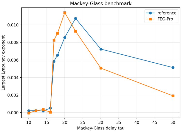
By constructing autocorrelation-guided sparse histories and performing distance-weighted k-nearest-neighbor multi-horizon forecasting on scalar time series, the method extracts a finite-horizon forecast-error growth slope lambda_FEG that approximates the dominant instability rate whenever the error-growth curve supports a quasi-linear regime, as demonstrated through agreement with known exponents on chaotic maps, Mackey-Glass delay dynamics, and Lorenz-63 observables.
What carries the argument
The forecast-error growth profile and its quasi-linear-regime slope lambda_FEG, obtained from geometrically averaged logarithmic errors after distance-weighted k-nearest-neighbor prediction.
If this is right
- In quasi-linear regimes the extracted slope provides a usable numerical estimate of the largest Lyapunov exponent from scalar data alone.
- Secondary profile descriptors including curvature, residual roughness after quadratic fit, monotonicity, and forecast-error distribution entropy serve as built-in diagnostics for the slope reliability.
- These same descriptors function as candidate features for machine-learning tasks in nonlinear signal classification.
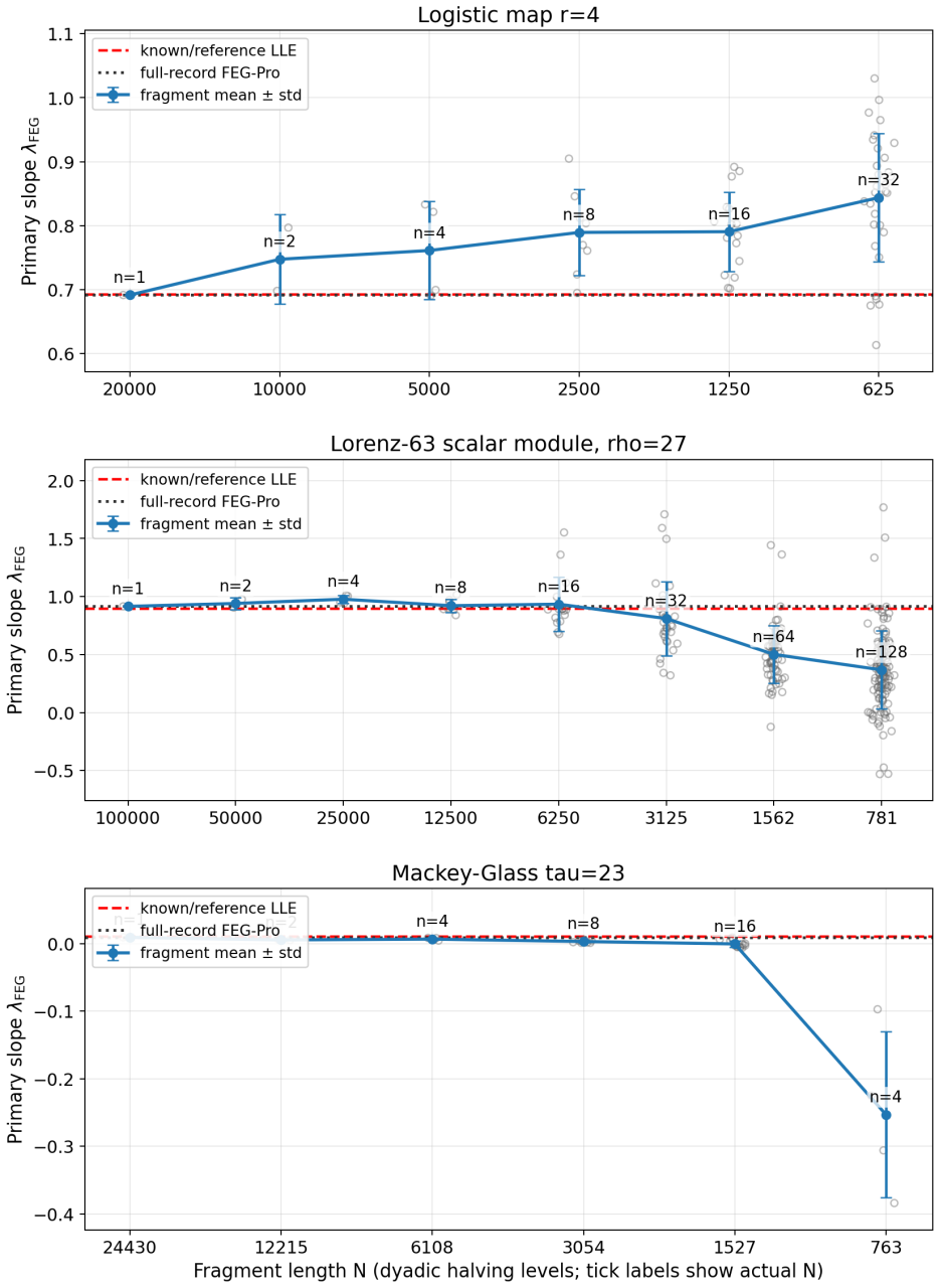
- The method remains interpretable under progressive record-length reduction, with roughness and mean error entropy often changing monotonically even when the slope itself becomes variable.
Where Pith is reading between the lines
- The profile approach could extend instability analysis to experimental time series from partially observed physical systems where only one variable is recorded.
- Combining the slope with the entropy and roughness descriptors might improve automated detection of transitions between regular and chaotic regimes in long records.
- Applying the pipeline to non-stationary data with slow parameter drifts could reveal how instability rates evolve over time without requiring model retraining.
Load-bearing premise
The distance-weighted nearest-neighbor forecasting step accurately captures the local expansion rates present in the underlying dynamics.
What would settle it
A systematic comparison in which lambda_FEG deviates markedly from the known largest Lyapunov exponent on a system whose error-growth curve displays a clear quasi-linear segment over several decades of horizon length.
Figures


read the original abstract
Estimating the largest Lyapunov exponent from a scalar time series is difficult when the governing equations, tangent dynamics, and full state vector are unavailable. We propose FEG-Pro, a forecast-error growth profiling framework for nonlinear scalar time series. The method constructs autocorrelation-guided sparse histories, performs distance-weighted k-nearest-neighbor multi-horizon forecasting, and analyzes the logarithmic growth of geometrically averaged forecast errors. Its primary output is the finite-horizon forecast-error growth slope, lambda_FEG. When the error-growth curve supports a quasi-linear regime, this slope can be compared with reference largest Lyapunov exponents as an estimate of the dominant instability rate. The same pipeline also extracts the formal fit-selection regime, curvature, residual roughness after quadratic detrending, monotonicity, and forecast-error distribution entropy (FEDE) from signed multi-horizon errors. These secondary descriptors are intended not only as diagnostic controls for the slope, but also as candidate machine-learning features for nonlinear signal analysis, because they encode profile geometry and distributional uncertainty not captured by lambda_FEG alone. We evaluate the method on chaotic maps, Mackey-Glass delay dynamics, and scalar Lorenz-63 observables with known or reference exponents. Full-record experiments show good agreement in quasi-linear cases and meaningful curve-shape information in curved or weak profiles. A dyadic length-halving experiment on representative logistic, Mackey-Glass, and Lorenz records shows that residual roughness and mean FEDE often change monotonically and remain interpretable as record length decreases, even when the slope becomes biased or highly variable. The results support treating forecast-error growth as a structured profile and feature-generation framework rather than a single-number estimator.
Editorial analysis
A structured set of objections, weighed in public.
Referee Report
Summary. The paper introduces FEG-Pro, a forecast-error growth profiling framework for nonlinear scalar time series. It constructs autocorrelation-guided sparse histories, applies distance-weighted k-nearest-neighbor multi-horizon forecasting, and extracts the finite-horizon forecast-error growth slope lambda_FEG from the logarithmic growth of geometrically averaged forecast errors. When a quasi-linear regime is present, lambda_FEG is proposed as an estimate of the largest Lyapunov exponent. Secondary descriptors including curvature, residual roughness, monotonicity, and forecast-error distribution entropy (FEDE) are also derived for diagnostics and as machine-learning features. Evaluations on chaotic maps, Mackey-Glass delay dynamics, and scalar Lorenz-63 observables report good agreement in quasi-linear cases and interpretable changes under dyadic length-halving.
Significance. If rigorously validated, the approach could supply a practical data-driven route to dominant instability rates from scalar observations when equations and full-state vectors are unavailable. Treating the error-growth curve as a structured profile rather than a single-number estimator, together with the dyadic length-halving experiments that track monotonicity of roughness and FEDE, adds diagnostic value beyond conventional Lyapunov estimation. The secondary descriptors could serve as useful features for nonlinear signal classification.
major comments (2)
- [Abstract / Evaluation] Abstract and evaluation section: the statement that 'full-record experiments show good agreement in quasi-linear cases' supplies no quantitative metrics (e.g., mean absolute deviation, correlation, or tabulated lambda_FEG versus reference LLE values with error bars) for the logistic, Mackey-Glass, or Lorenz-63 examples. This absence is load-bearing for the central claim that lambda_FEG can be compared with reference largest Lyapunov exponents as an estimate of the dominant instability rate.
- [Method (forecasting procedure)] Method description of the forecasting procedure: distance-weighted kNN multi-horizon prediction forms a weighted average over neighbors selected by Euclidean distance in the autocorrelation-guided history. This averaging can damp the observed growth rate relative to the true local stretching factor whenever the neighbors exhibit curvature or separation. No analytic bound on the resulting bias in lambda_FEG nor an ablation that replaces kNN with exact local linearization (Jacobian or tangent map) on identical histories is provided, which directly affects the validity of equating the slope to the largest Lyapunov exponent.
minor comments (2)
- [Notation] The definition of lambda_FEG as the slope of the log-averaged forecast-error curve should be tied to an explicit equation number for reproducibility.
- [Figures] Error-growth figures would be clearer if they indicated the identified quasi-linear regime and included variability across realizations or parameter choices for k and the autocorrelation threshold.
Simulated Author's Rebuttal
We thank the referee for the constructive feedback and for acknowledging the potential utility of treating forecast-error growth as a structured profile. We address each major comment below, indicating planned revisions where appropriate.
read point-by-point responses
-
Referee: [Abstract / Evaluation] Abstract and evaluation section: the statement that 'full-record experiments show good agreement in quasi-linear cases' supplies no quantitative metrics (e.g., mean absolute deviation, correlation, or tabulated lambda_FEG versus reference LLE values with error bars) for the logistic, Mackey-Glass, or Lorenz-63 examples. This absence is load-bearing for the central claim that lambda_FEG can be compared with reference largest Lyapunov exponents as an estimate of the dominant instability rate.
Authors: We agree that quantitative support is needed to substantiate the claim of good agreement. In the revised manuscript we will add a dedicated table in the evaluation section reporting lambda_FEG values next to reference LLEs for the logistic map, Mackey-Glass, and Lorenz-63 cases. The table will include mean absolute deviations, Pearson correlations across multiple realizations, and error bars obtained from repeated runs with varied random seeds for neighbor selection. revision: yes
-
Referee: [Method (forecasting procedure)] Method description of the forecasting procedure: distance-weighted kNN multi-horizon prediction forms a weighted average over neighbors selected by Euclidean distance in the autocorrelation-guided history. This averaging can damp the observed growth rate relative to the true local stretching factor whenever the neighbors exhibit curvature or separation. No analytic bound on the resulting bias in lambda_FEG nor an ablation that replaces kNN with exact local linearization (Jacobian or tangent map) on identical histories is provided, which directly affects the validity of equating the slope to the largest Lyapunov exponent.
Authors: The concern about possible damping bias from neighbor averaging is well taken. Because FEG-Pro targets settings where governing equations and full-state Jacobians are unavailable, exact local linearization is not feasible in general. For the benchmark systems with known dynamics we will add an ablation that recomputes the growth slopes using local linear fits on the identical autocorrelation-guided histories and directly compares the resulting slopes to the kNN-based lambda_FEG. We will also expand the discussion to clarify that lambda_FEG is offered as a practical proxy whose validity is conditioned on the presence of a quasi-linear regime, rather than an exact dynamical equivalent. revision: partial
- Deriving a general analytic bound on the bias in lambda_FEG that would hold for arbitrary nonlinear maps and reconstruction parameters.
Circularity Check
No circularity: lambda_FEG defined directly from observable forecast-error slope without reduction to inputs or self-citations
full rationale
The paper introduces FEG-Pro as a data-driven pipeline that builds autocorrelation-guided histories, applies distance-weighted kNN multi-horizon forecasting, computes geometrically averaged forecast errors, and extracts lambda_FEG as the slope of their logarithmic growth in quasi-linear regimes. This slope is then compared empirically to reference Lyapunov exponents on known systems (logistic map, Mackey-Glass, Lorenz-63). No equation or step equates lambda_FEG to the largest Lyapunov exponent by algebraic construction, fitted-parameter renaming, or load-bearing self-citation; the comparison is presented as an empirical approximation supported by experiments rather than a tautological identity. Secondary descriptors (curvature, FEDE, roughness) are likewise extracted directly from the same error profiles without circular re-use of the target quantity. The derivation chain remains self-contained against external benchmarks.
Axiom & Free-Parameter Ledger
free parameters (2)
- k (number of neighbors)
- autocorrelation threshold or lag set for sparse histories
axioms (1)
- domain assumption A quasi-linear regime exists in the forecast-error growth curve for the systems under study and its slope approximates the largest Lyapunov exponent.
Lean theorems connected to this paper
-
IndisputableMonolith/Foundation/RealityFromDistinction.leanreality_from_one_distinction unclear?
unclearRelation between the paper passage and the cited Recognition theorem.
The method constructs autocorrelation-guided sparse histories, performs distance-weighted k-nearest-neighbor multi-horizon forecasting, and analyzes the logarithmic growth of geometrically averaged forecast errors. Its primary output is the finite-horizon forecast-error growth slope, λ_FEG.
-
IndisputableMonolith/Cost/FunctionalEquation.leanwashburn_uniqueness_aczel unclear?
unclearRelation between the paper passage and the cited Recognition theorem.
When the error-growth curve supports a quasi-linear regime, this slope can be compared with reference largest Lyapunov exponents
What do these tags mean?
- matches
- The paper's claim is directly supported by a theorem in the formal canon.
- supports
- The theorem supports part of the paper's argument, but the paper may add assumptions or extra steps.
- extends
- The paper goes beyond the formal theorem; the theorem is a base layer rather than the whole result.
- uses
- The paper appears to rely on the theorem as machinery.
- contradicts
- The paper's claim conflicts with a theorem or certificate in the canon.
- unclear
- Pith found a possible connection, but the passage is too broad, indirect, or ambiguous to say the theorem truly supports the claim.
Reference graph
Works this paper leans on
-
[1]
Takens, Detecting strange attractors in turbulence, Lecture Notes in Mathematics 898 (1981) 366–381
F. Takens, Detecting strange attractors in turbulence, Lecture Notes in Mathematics 898 (1981) 366–381
work page 1981
-
[2]
A. Wolf, J. B. Swift, H. L. Swinney, J. A. Vastano, Determining lyapunov exponents from a time series, Physica D: Nonlinear Phenomena 16 (3) (1985) 285–317. 28
work page 1985
-
[3]
M. T. Rosenstein, J. J. Collins, C. J. De Luca, A practical method for calculating largest lyapunov exponents from small data sets, Physica D: Nonlinear Phenomena 65 (1–2) (1993) 117–134
work page 1993
-
[4]
H. Kantz, A robust method to estimate the maximal lyapunov exponent of a time series, Physics Letters A 185 (1) (1994) 77–87
work page 1994
-
[5]
H. D. I. Abarbanel, Analysis of Observed Chaotic Data, Springer, 1996
work page 1996
-
[6]
U. Parlitz, Estimating lyapunov exponents from time series, Chaos Detection and Pre- dictability (2016) 1–34doi:10.1007/978-3-662-48410-4_1
-
[7]
A. M. Fraser, H. L. Swinney, Independent coordinates for strange attractors from mutual information, Physical Review A 33 (2) (1986) 1134–1140
work page 1986
-
[8]
M. B. Kennel, R. Brown, H. D. I. Abarbanel, Determining embedding dimension for phase-space reconstruction using a geometrical construction, Physical Review A 45 (6) (1992) 3403–3411
work page 1992
-
[9]
H. Ma, C.-z. Han, Selection of embedding dimension and delay time in phase space reconstruction, Frontiers of Electrical and Electronic Engineering in China 1 (2006) 111–114.doi:10.1007/s11460-005-0023-7
-
[10]
M. Matilla-García, I. Morales, J. Rodríguez, M. R. Marín, Selection of embedding di- mension and delay time in phase space reconstruction via symbolic dynamics, Entropy 23 (2) (2021) 221.doi:10.3390/e23020221
- [11]
-
[12]
S. Zhu, L. Gan, Incomplete phase-space method to reveal time delay from scalar time series, Physical Review E 94 (5) (2016) 052210.doi:10.1103/physreve.94.052210
-
[13]
X. Zeng, R. Eykholt, R. A. Pielke, Estimating the lyapunov-exponent spectrum from short time series of low precision, Physical Review Letters 66 (25) (1991) 3229–3232. doi:10.1103/physrevlett.66.3229
-
[14]
H.-f. Liu, Z. Dai, W.-f. Li, X. Gong, Z.-h. Yu, Noise robust estimates of the largest lyapunov exponent, Physics Letters A 341 (2005) 119–127.doi:10.1016/j.physleta. 2005.04.048
-
[15]
T.-L. Yao, H.-f. Liu, J.-L. Xu, W.-f. Li, Estimating the largest lyapunov exponent and noise level from chaotic time series, Chaos 22 (3) (2012) 033102.doi:10.1063/1. 4731800
work page doi:10.1063/1 2012
-
[16]
S. Mehdizadeh, M. A. Sanjari, Effect of noise and filtering on largest lyapunov exponent of time series associated with human walking, Journal of Biomechanics 64 (2017) 236– 239.doi:10.1016/j.jbiomech.2017.09.009. 29
-
[17]
S. Mehdizadeh, A robust method to estimate the largest lyapunov exponent of noisy signals: A revision to the rosenstein’s algorithm, bioRxiv (2018).doi:10.1101/381111
-
[18]
L. Escot, J. E. Sandubete, Estimating lyapunov exponents on a noisy environment by global and local jacobian indirect algorithms, Applied Mathematics and Computation 436 (2023) 127498.doi:10.1016/j.amc.2022.127498
-
[19]
J. D. Farmer, J. J. Sidorowich, Predicting chaotic time series, Physical Review Letters 59 (8) (1987) 845–848.doi:10.1103/physrevlett.59.845
-
[20]
M. Casdagli, Nonlinear prediction of chaotic time series, Physica D: Nonlinear Phenom- ena 35 (1989) 335–356.doi:10.1016/0167-2789(89)90074-2
-
[21]
G. Sugihara, R. M. May, Nonlinear forecasting as a way of distinguishing chaos from measurement error in time series, Nature 344 (1990) 734–741.doi:10.1038/344734a0
-
[22]
R. Hegger, H. Kantz, T. Schreiber, Practical implementation of nonlinear time series methods: The tisean package, Chaos 9 (2) (1999) 413–435.doi:10.1063/1.166424
- [23]
-
[24]
G. Sugihara, Nonlinear forecasting for the classification of natural time series, Philo- sophical Transactions of the Royal Society of London. Series A 348 (1994) 477–495. doi:10.1098/rsta.1994.0106
-
[25]
C.-W. Chang, M. Ushio, C.-h. Hsieh, Empirical dynamic modeling for beginners, Eco- logical Research 32 (2017) 785–796.doi:10.1007/s11284-017-1469-9
-
[26]
E. Bradley, H. Kantz, Nonlinear time-series analysis revisited, Chaos 25 (9) (2015) 097610.doi:10.1063/1.4917289
-
[27]
B. D. Fulcher, Feature-based time-series analysis, Feature Engineering for Machine Learning and Data Analytics (2017) 87–116doi:10.1201/9781315181080-4
-
[28]
C. H. Lubba, S. S. Sethi, P. Knaute, S. R. Schultz, B. D. Fulcher, N. S. Jones, catch22: Canonical time-series characteristics, Data Mining and Knowledge Discovery 33 (2019) 1821–1852.doi:10.1007/s10618-019-00647-x
-
[29]
M. Christ, N. Braun, J. Neuffer, A. W. Kempa-Liehr, Time series feature extraction on basis of scalable hypothesis tests (tsfresh - a python package), Neurocomputing 307 (2018) 72–77.doi:10.1016/j.neucom.2018.03.067
-
[30]
T. Henderson, B. D. Fulcher, Feature-based time-series analysis in r using the theft package, arXiv abs/2208.06146 (2022).doi:10.48550/arxiv.2208.06146
-
[31]
J. F. L. de Oliveira, E. Silva, P. S. G. de Mattos Neto, A hybrid system based on dynamic selection for time series forecasting, IEEE Transactions on Neural Networks and Learning Systems 33 (2021) 3251–3263.doi:10.1109/tnnls.2021.3051384. 30
-
[32]
E. Ilhan, A. B. Koc, S. S. Kozat, Exploiting residual errors in nonlinear online prediction, Machine Learning 113 (2024) 6065–6091.doi:10.1007/s10994-024-06554-7
-
[33]
V. Jensen, F. Bianchi, S. N. Anfinsen, Ensemble conformalized quantile regression for probabilistic time series forecasting, IEEE Transactions on Neural Networks and Learn- ing Systems 35 (2022) 9014–9025.doi:10.1109/tnnls.2022.3217694
- [34]
-
[35]
C. E. Shannon, A mathematical theory of communication, The Bell System Technical Journal 27 (3) (1948) 379–423
work page 1948
-
[36]
R. Guntu, P. K. Yeditha, M. Rathinasamy, M. Perc, N. Marwan, J. Kurths, A. Agarwal, Wavelet entropy-based evaluation of intrinsic predictability of time series, Chaos 30 (3) (2020) 033117.doi:10.1063/1.5145005
-
[37]
G. A. Papacharalampous, H. Tyralis, I. Pechlivanidis, S. Grimaldi, E. Volpi, Massive feature extraction for explaining and foretelling hydroclimatic time series forecastability at the global scale, Geoscience Frontiers 13 (2022) 101349.doi:10.1016/j.gsf.2022. 101349
-
[38]
A. Velichko, M. Belyaev, P. Boriskov, A novel approach for estimating largest lyapunov exponents in one-dimensional chaotic time series using machine learning, Chaos 35 (10) (2025).doi:10.1063/5.0289352
-
[39]
M. Belyaev, A. Velichko, V. Putrolaynen, Forecasting chaotic time series using echo state networks: Limits of predictability and relationship with entropy, in: Proceedings of SPIE, Vol. 13803, 2025, p. 138031C.doi:10.1117/12.3078206
-
[40]
Y. Muruganantham, A. Velichko, S. Rajendran, Local lyapunov analysis via micro- ensembles: Finite-time lyapunov exponent estimation and knn-based predictive com- parison in complex-valued bam neural networks (2025)
work page 2025
-
[41]
M. Shams, A. Velichko, B. Carpentieri, Optimizing parallel schemes with lyapunov ex- ponents and knn-lle estimation, arXiv abs/2601.13604 (2026).doi:10.48550/arxiv. 2601.13604
work page internal anchor Pith review doi:10.48550/arxiv 2026
-
[42]
M. C. Mackey, L. Glass, Oscillation and chaos in physiological control systems, Science 197 (4300) (1977) 287–289
work page 1977
-
[43]
E. N. Lorenz, Deterministic nonperiodic flow, Journal of the Atmospheric Sciences 20 (2) (1963) 130–141. 31
work page 1963
discussion (0)
Sign in with ORCID, Apple, or X to comment. Anyone can read and Pith papers without signing in.