Random spanning tree Markov random field priors for Bayesian inverse problems in imaging
Pith reviewed 2026-05-20 08:25 UTC · model grok-4.3
The pith
Random spanning trees as hyperpriors on pixel grids let Bayesian imaging regularize only a sparse random subset of edges, preserving contrast better than standard difference Markov random fields.
A machine-rendered reading of the paper's core claim, the machinery that carries it, and where it could break.
Core claim
Placing a hyperprior on the connectivity graph of the pixel grid in the form of a random spanning tree couples discrete and continuous variables so that only a sparse random subset of edges is regularized. This structure preserves edges in the image with reduced contrast loss compared to standard difference-based Markov random fields while still allowing efficient posterior sampling via a Gibbs sampler that alternates tree and pixel updates.
What carries the argument
Random spanning tree hyperprior on the pixel-grid graph, which supplies a minimal connected subset of edges to which difference distributions are applied.
If this is right
- Only a minimal connected subset of neighboring differences receives regularization in each sample, reducing the cumulative smoothing across edges.
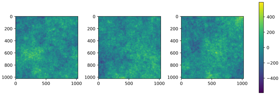
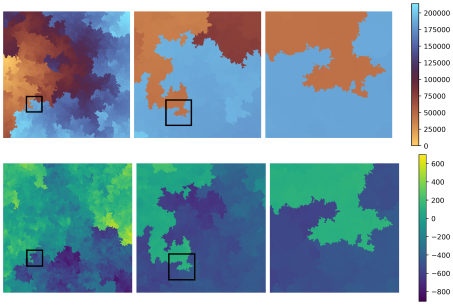
- High-resolution draws from the prior exhibit fractal-like interfaces induced by the random tree connectivity.
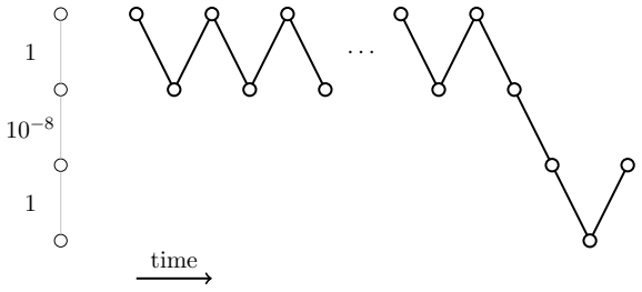
- The Gibbs sampler jointly updates the discrete tree structure and the continuous image values to explore the posterior.
- The prior is applied to standard restoration tasks including denoising, deblurring, and inpainting.
Where Pith is reading between the lines
- The same tree-structured sparsity mechanism could be tested on inverse problems defined on irregular meshes rather than regular grids.
- Because the interfaces are fractal, the method invites quantitative study of whether those patterns affect downstream perceptual or task-specific metrics.
- Combining the spanning-tree hyperprior with learned difference distributions might further tune the balance between smoothness and edge fidelity.
Load-bearing premise
Jointly sampling the random spanning tree and the pixel values yields reconstructions that outperform standard MRF priors on real inverse problems without introducing visible artifacts from the fractal-like interfaces.
What would settle it
A side-by-side reconstruction of a test image containing known sharp discontinuities in which the random-tree prior produces measurably lower edge contrast or new fractal artifacts relative to a standard Laplace difference prior would falsify the performance claim.
Figures


read the original abstract
Markov random fields are common prior distributions used in Bayesian inverse imaging problems. In particular, difference priors assign probability distributions to differences between neighbouring pixels, such as Gaussian, Laplace, or Cauchy distributions. Depending on the chosen difference distribution, these priors have smoothing or edge-preserving properties. In this work, we propose a hyperprior on the connectivity graph of the pixel grid in the form of a random spanning tree, i.e., a random connected graph with the minimal number of edges, thereby coupling continuous and discrete random variables in the prior. By using random spanning trees, only a sparse random subset of edges is regularized, which helps preserve edges in the image with reduced contrast loss compared to standard difference-based Markov random fields. We discuss how fractal-like interfaces arise in high-resolution prior samples due to the random-tree connectivity. Finally, we propose a Gibbs sampler that alternates between the discrete tree updates and continuous pixel updates to efficiently explore the posterior distribution. We apply the method to various standard test image restoration problems, including denoising, deblurring, and inpainting, to study the impact of the proposed prior in comparison with existing Markov random fields.
Editorial analysis
A structured set of objections, weighed in public.
Referee Report
Summary. The manuscript proposes a novel Markov random field prior for Bayesian inverse problems in imaging by placing a hyperprior on the pixel-grid connectivity graph in the form of a random spanning tree. This couples discrete tree variables with continuous pixel intensities so that only a sparse random subset of edges is regularized, with the goal of preserving edges while incurring less contrast loss than standard difference-based MRFs. The authors note the appearance of fractal-like interfaces in high-resolution prior samples, introduce a Gibbs sampler that alternates between tree and pixel updates, and apply the method to standard denoising, deblurring, and inpainting test problems.
Significance. If the claimed reduction in contrast loss is realized without visible artifacts from the fractal interfaces, the construction would provide a principled way to randomize the support of an MRF prior and could influence the design of structure-preserving priors more broadly. The explicit coupling of discrete graph variables with continuous image variables and the associated Gibbs sampler constitute a technically coherent contribution.
major comments (2)
- [§4] §4 (discussion of fractal-like interfaces): the manuscript correctly observes that high-resolution prior samples exhibit fractal-like interfaces due to the random-tree connectivity, yet provides no quantitative posterior analysis or metric (e.g., edge-sharpness histograms or boundary artifact scores) demonstrating that these interfaces are suppressed by the data likelihood or do not degrade reconstructions on the reported test problems. This directly affects the central claim that sparse random regularization yields reduced contrast loss.
- [§6] §6 (numerical experiments): the comparisons with standard Laplace and Gaussian MRFs report only conventional error metrics (PSNR/SSIM) and visual results; no ablation isolating the effect of the random spanning-tree hyperprior on contrast loss (for example, via gradient-magnitude distributions or boundary-contrast ratios) is presented, leaving the principal advantage unverified.
minor comments (2)
- [§3] The probability measure over spanning trees (Eq. (3) or equivalent) should be written explicitly rather than described only in prose, to clarify the normalization constant.
- Figure captions for prior samples should state the grid resolution and number of trees drawn so that the fractal-interface observation can be reproduced.
Simulated Author's Rebuttal
We thank the referee for the constructive comments and the positive assessment of the technical contribution. We address each major comment below and indicate planned revisions to strengthen the manuscript.
read point-by-point responses
-
Referee: [§4] §4 (discussion of fractal-like interfaces): the manuscript correctly observes that high-resolution prior samples exhibit fractal-like interfaces due to the random-tree connectivity, yet provides no quantitative posterior analysis or metric (e.g., edge-sharpness histograms or boundary artifact scores) demonstrating that these interfaces are suppressed by the data likelihood or do not degrade reconstructions on the reported test problems. This directly affects the central claim that sparse random regularization yields reduced contrast loss.
Authors: We agree that the manuscript would benefit from quantitative posterior analysis to confirm suppression of fractal-like interfaces. Section 4 discusses these structures only for prior samples, while Section 6 relies on visual inspection of reconstructions to argue that they do not degrade results. The data likelihood is expected to suppress such artifacts, but we acknowledge the absence of explicit metrics. In the revision we will add quantitative measures, such as edge-sharpness histograms and boundary-contrast ratios computed on posterior means for the test problems, to directly support the claim. revision: yes
-
Referee: [§6] §6 (numerical experiments): the comparisons with standard Laplace and Gaussian MRFs report only conventional error metrics (PSNR/SSIM) and visual results; no ablation isolating the effect of the random spanning-tree hyperprior on contrast loss (for example, via gradient-magnitude distributions or boundary-contrast ratios) is presented, leaving the principal advantage unverified.
Authors: The referee is correct that the experiments do not include a direct ablation isolating the effect on contrast loss. Current results rely on PSNR/SSIM and visual comparisons, which show competitive or improved performance with better edge preservation. To verify the principal advantage, we will add in the revised Section 6 an analysis of gradient-magnitude distributions and boundary-contrast ratios across the different priors on the reported test problems. revision: yes
Circularity Check
No significant circularity; derivation is self-contained
full rationale
The paper defines a novel prior by placing a hyperprior on the pixel-grid connectivity in the form of a random spanning tree, directly coupling discrete tree variables to continuous pixel values via the proposed joint distribution. The central construction, the Gibbs sampler alternating between tree and pixel updates, and the claimed edge-preservation benefit are all introduced as new elements without reducing to fitted parameters, self-referential equations, or load-bearing self-citations whose content is itself unverified. No step in the provided derivation chain equates a prediction or result to its own inputs by construction, and the model remains externally falsifiable through the described image-restoration experiments.
Axiom & Free-Parameter Ledger
axioms (1)
- domain assumption Pixel grids can be treated as undirected graphs whose edges represent candidate difference penalties.
invented entities (1)
-
Random spanning tree hyperprior
no independent evidence
Lean theorems connected to this paper
-
IndisputableMonolith/Foundation/AlexanderDuality.leanalexander_duality_circle_linking unclear?
unclearRelation between the paper passage and the cited Recognition theorem.
By using random spanning trees, only a sparse random subset of edges is regularized... fractal-like interfaces arise in high-resolution prior samples due to the random-tree connectivity... chordal Schramm-Loewner evolution (SLE κ) with κ=2, which almost surely has fractal dimension 1.25.
What do these tags mean?
- matches
- The paper's claim is directly supported by a theorem in the formal canon.
- supports
- The theorem supports part of the paper's argument, but the paper may add assumptions or extra steps.
- extends
- The paper goes beyond the formal theorem; the theorem is a base layer rather than the whole result.
- uses
- The paper appears to rely on the theorem as machinery.
- contradicts
- The paper's claim conflicts with a theorem or certificate in the canon.
- unclear
- Pith found a possible connection, but the passage is too broad, indirect, or ambiguous to say the theorem truly supports the claim.
Reference graph
Works this paper leans on
-
[1]
D. Aldous and J. A. Fill. Reversible markov chains and random walks on graphs, 2002. Unfinished monograph, recompiled 2014, available athttp://www.stat.berkeley.edu/ $\sim$aldous/RWG/book.html
work page 2002
-
[2]
D. J. Aldous. Lower bounds for covering times for reversible Markov chains and random walks on graphs.Journal of Theoretical Probability, 2(1):91–100, 1989
work page 1989
-
[3]
D. J. Aldous. The random walk construction of uniform spanning trees and uniform labelled trees.SIAM Journal on Discrete Mathematics, 3(4):450–465, 1990
work page 1990
-
[4]
R. Aleliunas, R. M. Karp, R. J. Lipton, L. Lov´ asz, and C. Rackoff. Random walks, universal traversal sequences, and the complexity of maze problems. InProceedings of the 20th Annual Symposium on Foundations of Computer Science, pages 218–223, 1979
work page 1979
-
[5]
J. M. Bardsley. Laplace-distributed increments, the Laplace prior, and edge-preserving regularization.Journal of Inverse & Ill-Posed Problems, 20(3), 2012
work page 2012
-
[6]
J. M. Bardsley. Mcmc-based image reconstruction with uncertainty quantification.SIAM Journal on Scientific Computing, 34(3):A1316–A1332, 2012
work page 2012
-
[7]
V. Beffara. The dimension of the SLE curves.The Annals of Probability, pages 1421–1452, 2008
work page 2008
- [8]
-
[9]
A. Z. Broder. Generating random spanning trees. InFOCS, volume 89, pages 442–447, 1989
work page 1989
-
[10]
D. A. Brown, C. S. McMahan, and S. Watson Self. Sampling strategies for fast updating of Gaussian Markov random fields.The American Statistician, 75(1):52–65, 2021
work page 2021
-
[11]
L. L. Duan and D. B. Dunson. Bayesian spanning tree: estimating the backbone of the dependence graph.Journal of Machine Learning Research, 24(397):1–44, 2023
work page 2023
- [12]
-
[13]
A. Gelman. Prior distributions for variance parameters in hierarchical models (comment on article by Browne and Draper).Bayesian Analysis, 1:515–533, 2006. 21
work page 2006
-
[14]
C. Hans, A. Dobra, and M. West. Shotgun stochastic search for “large p” regression. Journal of the American Statistical Association, 102(478):507–516, 2007
work page 2007
- [15]
-
[16]
J. P. Kaipio and E. Somersalo.Statistical and computational inverse problems. Springer, 2005
work page 2005
-
[17]
H. Kekkonen, M. Lassas, E. Saksman, and S. Siltanen. Random tree Besov priors–towards fractal imaging.Inverse Problems and Imaging, 17(2):507–531, 2023
work page 2023
-
[18]
H. Kekkonen and A. Tataris. Random tree Besov priors: Data-driven regularisation pa- rameter selection.arXiv preprint arXiv:2601.12957, 2026
-
[19]
V. Kolmogorov, T. Pock, and M. Rolinek. Total variation on a tree.SIAM Journal on Imaging Sciences, 9(2):605–636, 2016
work page 2016
-
[20]
J. B. Kruskal. On the shortest spanning subtree of a graph and the traveling salesman problem.Proceedings of the American Mathematical society, 7(1):48–50, 1956
work page 1956
-
[21]
M. Lassas and S. Siltanen. Can one use total variation prior for edge-preserving Bayesian inversion?Inverse problems, 20(5):1537, 2004
work page 2004
-
[22]
G. F. Lawler, O. Schramm, and W. Werner. Conformal invariance of planar loop-erased random walks and uniform spanning trees. InSelected Works of Oded Schramm, pages 931–987. Springer, 2011
work page 2011
-
[23]
R. Lazimy. Mixed-integer quadratic programming.Mathematical Programming, 22(1):332– 349, 1982
work page 1982
-
[24]
R. Lyons and Y. Peres.Probability on trees and networks, volume 42. Cambridge University Press, 2017
work page 2017
-
[25]
M. Markkanen, L. Roininen, J. M. Huttunen, and S. Lasanen. Cauchy difference priors for edge-preserving Bayesian inversion.Journal of Inverse and Ill-posed Problems, 27(2):225– 240, 2019
work page 2019
-
[26]
T. Park and G. Casella. The Bayesian lasso.Journal of the american statistical association, 103(482):681–686, 2008
work page 2008
-
[27]
R. C. Prim. Shortest connection networks and some generalizations.The Bell System Technical Journal, 36(6):1389–1401, 1957
work page 1957
-
[28]
J. G. Propp and D. B. Wilson. How to get a perfectly random sample from a generic Markov chain and generate a random spanning tree of a directed graph.Journal of Algorithms, 27(2):170–217, 1998
work page 1998
- [29]
-
[30]
O. Schramm and S. Sheffield. Contour lines of the two-dimensional discrete Gaussian free field.Acta Math, 202:21–137, 2009
work page 2009
-
[31]
A. Schreck, G. Fort, S. Le Corff, and E. Moulines. A shrinkage-thresholding Metropolis adjusted Langevin algorithm for Bayesian variable selection.IEEE Journal of Selected Topics in Signal Processing, 10(2):366–375, 2015. 22
work page 2015
-
[32]
A. Senchukova, F. Uribe, and L. Roininen. Bayesian inversion with Students’ t priors based on Gaussian scale mixtures.Inverse Problems, 40(10):105013, 2024
work page 2024
-
[33]
V. K. Shante and S. Kirkpatrick. An introduction to percolation theory.Advances in Physics, 20(85):325–357, 1971
work page 1971
- [34]
-
[35]
S. Siltanen, V. Kolehmainen, S. J¨ arvenp¨ a¨ a, J. P. Kaipio, P. Koistinen, M. Lassas, J. Pirttil¨ a, and E. Somersalo. Statistical inversion for medical x-ray tomography with few radiographs: I. General theory.Physics in Medicine & Biology, 48(10):1437, 2003
work page 2003
-
[36]
J. Suuronen, N. K. Chada, and L. Roininen. Cauchy Markov random field priors for Bayesian inversion.Statistics and computing, 32(2):33, 2022
work page 2022
-
[37]
E. Tam, D. B. Dunson, and L. L. Duan. Exact sampling of spanning trees via fast-forwarded random walks.Biometrika, 112(2):asaf031, 2025
work page 2025
- [38]
-
[39]
P. Virtanen, R. Gommers, T. E. Oliphant, M. Haberland, T. Reddy, D. Cournapeau, E. Burovski, P. Peterson, W. Weckesser, J. Bright, S. J. van der Walt, M. Brett, J. Wilson, K. J. Millman, N. Mayorov, A. R. J. Nelson, E. Jones, R. Kern, E. Larson, C. J. Carey, ˙I. Polat, Y. Feng, E. W. Moore, J. VanderPlas, D. Laxalde, J. Perktold, R. Cimrman, I. Henriksen,...
work page 2020
-
[40]
M. Vono, N. Dobigeon, and P. Chainais. High-dimensional Gaussian sampling: A review and a unifying approach based on a stochastic proximal point algorithm.SIAM Review, 64(1):3–56, 2022
work page 2022
-
[41]
D. B. Wilson. Generating random spanning trees more quickly than the cover time. In Proceedings of the twenty-eighth annual ACM symposium on Theory of computing, pages 296–303, 1996. 23
work page 1996
discussion (0)
Sign in with ORCID, Apple, or X to comment. Anyone can read and Pith papers without signing in.