End-to-End PDE-Based Quantum Algorithms for Multi-Asset Option Pricing under Local and Stochastic Volatility
Pith reviewed 2026-06-29 17:23 UTC · model grok-4.3
The pith
Quantum algorithms solve multi-asset option pricing PDEs with polynomial speedup over classical grids.
A machine-rendered reading of the paper's core claim, the machinery that carries it, and where it could break.
Core claim
After finite-difference discretization of the pricing PDEs on spatial grids, standard quantum linear-system solvers achieve end-to-end gate complexity with leading dependence tilde-O(d squared N to the power 2 plus d over 2) for local-volatility Black-Scholes and tilde-O(d squared N to the d plus 2) for Heston; these scalings correspond to polynomial improvement factors N to the d over 2 and N to the d over grid-based finite-difference baselines.
What carries the argument
End-to-end quantum linear-system solver applied to the finite-difference discretization of the multi-dimensional pricing PDE, which carries the argument from classical input data to classical output prices with the stated gate counts.
If this is right
- Single-point option values can be recovered with gate cost that grows only polynomially rather than exponentially in the number of assets d.
- The Heston instance of the framework recovers prices across multiple strikes together with the implied-volatility smile or skew.
- The reported gate counts translate to Clifford+T resources by standard compilation without changing the leading scaling.
- Numerical benchmarks confirm that the quantum-derived prices match those obtained from classical solvers on the same discretizations.
Where Pith is reading between the lines
- The same discretization-plus-solver pipeline could be reused for other parabolic PDEs in finance provided the matrix sparsity pattern remains comparable.
- Practical advantage on near-term hardware would still require the overhead of error correction to stay within the same polynomial envelope.
- The multi-asset grid structure may introduce fill-in or conditioning effects that alter the precise exponent once the solver is instantiated on a concrete quantum architecture.
Load-bearing premise
After finite-difference discretization of the pricing PDEs on spatial grids, standard quantum linear-system solvers achieve the stated gate complexities with no model-specific overheads or additional costs from the multi-asset structure.
What would settle it
An explicit gate-count analysis of the quantum linear solver on the concrete sparse matrices produced by the multi-asset local-volatility or Heston discretizations that exceeds the claimed leading scaling by more than polylog factors.
Figures


read the original abstract
Multi-asset option pricing under local- and stochastic-volatility models leads naturally to high-dimensional parabolic PDEs. We develop an end-to-end quantum PDE framework for European option pricing under local-volatility Black--Scholes and Heston models. The framework takes classical contract and model data as input and returns classical estimates of selected option values. We solve the pricing PDEs after finite-difference discretization on spatial grids. For $N=2^n$ grid points per spatial direction and $d$ assets, the end-to-end gate complexity for single-point recovery, counted in elementary CNOT gates and one-qubit Pauli-axis rotations, has leading grid-size dependence $\widetilde{O}(d^2 N^{2+d/2})$ for local-volatility Black--Scholes and $\widetilde{O}(d^2 N^{d+2})$ for Heston. Relative to grid-based finite-difference baselines, these scalings correspond to polynomial improvement factors $N^{d/2}$ and $N^d$, respectively. These estimates translate to Clifford+T resources via standard compilation. We complement the complexity analysis with numerical benchmarks against standard classical methods. In the Heston setting, the framework recovers option prices across strikes together with the associated implied-volatility smile/skew. Overall, this work provides a complete end-to-end quantum pricing pipeline with explicit resource accounting and theoretical performance guarantees.
Editorial analysis
A structured set of objections, weighed in public.
Referee Report
Summary. The manuscript develops an end-to-end quantum PDE framework for European multi-asset option pricing under local-volatility Black-Scholes and Heston models. After finite-difference discretization on N-point grids per dimension, it applies quantum linear-system solvers and reports end-to-end gate complexities (in CNOTs and Pauli rotations) with leading terms ilde{O}(d^2 N^{2+d/2}) and ilde{O}(d^2 N^{d+2}), respectively, claiming polynomial speedups over classical grid methods; the claims are accompanied by numerical benchmarks that recover prices and implied-volatility surfaces.
Significance. If the stated gate complexities are established with explicit block-encoding constructions and condition-number bounds that absorb all multi-asset overheads, the work would supply a concrete quantum pricing pipeline with reproducible resource estimates and benchmarks, strengthening the case for quantum advantage in high-dimensional financial PDEs.
major comments (1)
- [Complexity analysis] Complexity analysis section: the headline scalings ilde{O}(d^2 N^{2+d/2}) (local-vol BS) and ilde{O}(d^2 N^{d+2}) (Heston) are derived by invoking standard quantum linear-system solvers on the FD-discretized operators, yet no explicit sparsity pattern, block-encoding construction, or condition-number bound is supplied for the d-dimensional (or (d+1)-dimensional) stencil that includes cross-derivative terms; without these, it cannot be verified that the quoted leading terms already incorporate all multi-asset costs or that s = O(d^2) and \kappa = O(N^2) hold without additional poly(d) or log N factors.
minor comments (1)
- [Abstract] The abstract and introduction would benefit from a one-sentence pointer to the specific section containing the block-encoding and conditioning arguments.
Simulated Author's Rebuttal
We thank the referee for their careful reading and constructive feedback on the manuscript. The single major comment is addressed point-by-point below; we will revise the paper to supply the requested explicit details.
read point-by-point responses
-
Referee: [Complexity analysis] Complexity analysis section: the headline scalings ilde{O}(d^2 N^{2+d/2}) (local-vol BS) and ilde{O}(d^2 N^{d+2}) (Heston) are derived by invoking standard quantum linear-system solvers on the FD-discretized operators, yet no explicit sparsity pattern, block-encoding construction, or condition-number bound is supplied for the d-dimensional (or (d+1)-dimensional) stencil that includes cross-derivative terms; without these, it cannot be verified that the quoted leading terms already incorporate all multi-asset costs or that s = O(d^2) and \kappa = O(N^2) hold without additional poly(d) or log N factors.
Authors: We appreciate the referee highlighting the need for more explicit details. The headline scalings follow from applying standard quantum linear-system solvers to the FD-discretized operators. For both models the matrix is sparse with s = O(d^2) nonzeros per row: the local-volatility Black-Scholes operator contains O(d^2) second-derivative and cross-derivative terms, each contributing a constant-size stencil (at most 9 points per pair of coordinates), while the Heston operator adds one extra dimension but preserves the same per-row sparsity order. The condition number satisfies \kappa = O(N^2) for second-order FD discretizations of these uniformly elliptic operators on grids of spacing 1/N; the bound is independent of d once the explicit d^2 prefactor is extracted. Block-encodings of such sparse stencil matrices are constructed via standard sparse-access oracles (or linear-combination-of-unitaries), incurring only polylog(N,d) overhead absorbed in the ilde{O} notation. The manuscript invokes these standard facts without spelling out the constructions. To make the claims fully verifiable we will add an appendix containing (i) the explicit sparsity pattern of the multi-dimensional stencil with cross terms, (ii) a sketch of the block-encoding construction, and (iii) a self-contained reference or short derivation of the \kappa = O(N^2) bound. These additions will confirm that the quoted leading terms already incorporate all multi-asset costs without hidden poly(d) or extra log N factors. revision: yes
Circularity Check
No circularity; complexity claims rest on external standard QLS bounds after discretization
full rationale
The abstract and description present the gate complexities as direct consequences of applying standard quantum linear-system solvers to FD-discretized PDE operators on N^d grids, with leading terms ilde{O}(d^2 N^{2+d/2}) and ilde{O}(d^2 N^{d+2}). No self-definitional equations, fitted parameters renamed as predictions, or load-bearing self-citations appear. The derivation is self-contained against external QLS results (HHL-style solvers with stated sparsity/conditioning assumptions), satisfying the criteria for an independent claim.
Axiom & Free-Parameter Ledger
axioms (1)
- domain assumption Finite-difference discretization of the multi-asset pricing PDEs produces a linear system whose solution cost is governed by standard quantum linear-system algorithms.
Forward citations
Cited by 1 Pith paper
-
Quantum Derivative Pricing for SPDEs via BDSDE Representation
Quantum-accelerated MLMC methods for BDSDE-based SPDE derivative pricing and Greeks achieve sampling complexity improvement from O(ε^{-2}) to O(ε^{-1}).
Reference graph
Works this paper leans on
-
[1]
curse of dimensionality,
End-to-end complexity scaling We now state the end-to-end scaling for the multi-asset Black–Scholes pipeline, in a form consistent with the 1D summary in Appendix A.3. We use the Worst-of Call payoff state-preparation routine from Table VII, with its success probability boosted to O(1) using the amplification technique in Appendix J. The backward evolutio...
-
[2]
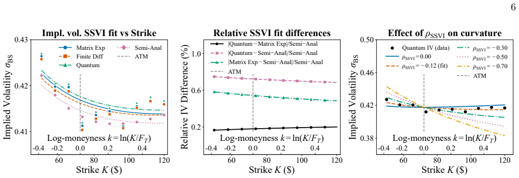
prices → implied vols
Implied-volatility slices in Heston: arbitrage-free regularization To compare Heston-generated prices (classical or quantum) away from the at-the-money (ATM) strike, we work with implied-volatility slices at fixed maturity. In practice, quoted strikes are sparse around ATM, and in our setting the inversion from prices to implied volatility is further corr...
-
[3]
Linear ODE system for Heston model The overall discretization pipeline is the same as in Appendix A.1 and B.2; in particular, we employ the standard second-order accurate centered finite-difference schemes summarized in Table III and Eq. (B8). The terminal payoff provides the initial condition for the backward-time evolution (or, equivalently, the termina...
-
[4]
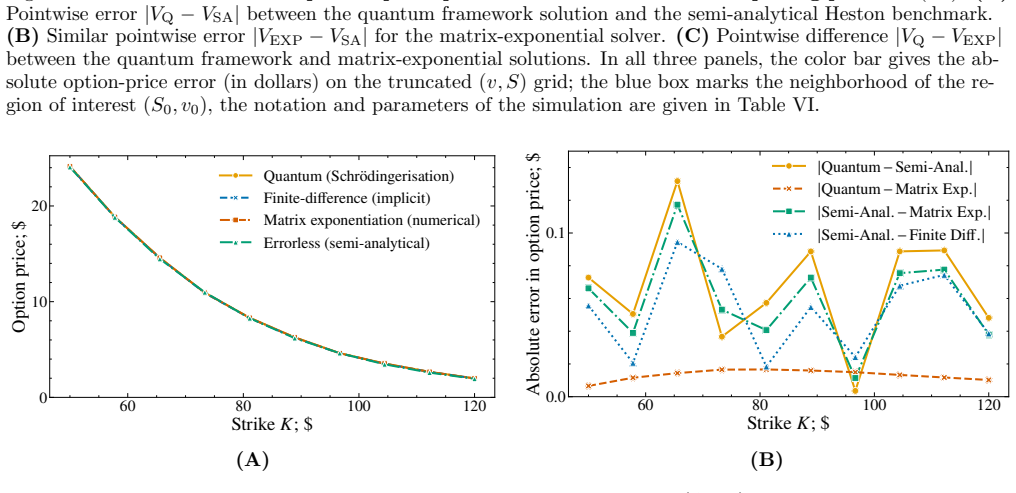
The purpose of these numerical tests is to verify that the quantum workflow produces results consistent with classical benchmarks and semi-analytical solutions
Numerical simulation This subsection demonstrates the application of the quantum framework developed in Appendices E–G to the one-asset Heston model (C3). The purpose of these numerical tests is to verify that the quantum workflow produces results consistent with classical benchmarks and semi-analytical solutions. Specifically, we compare the quantum 26 −...
-
[5]
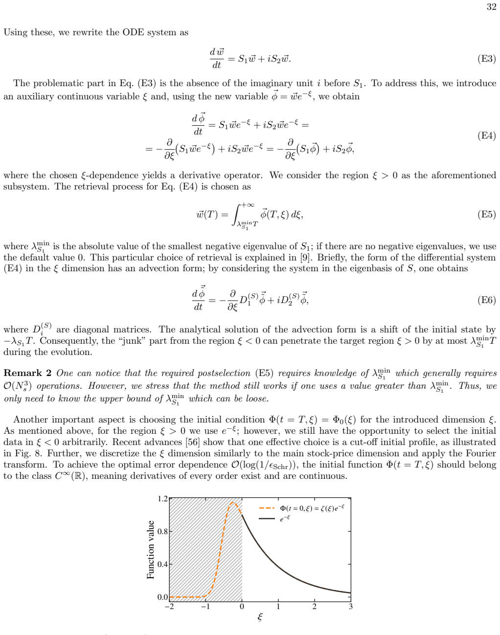
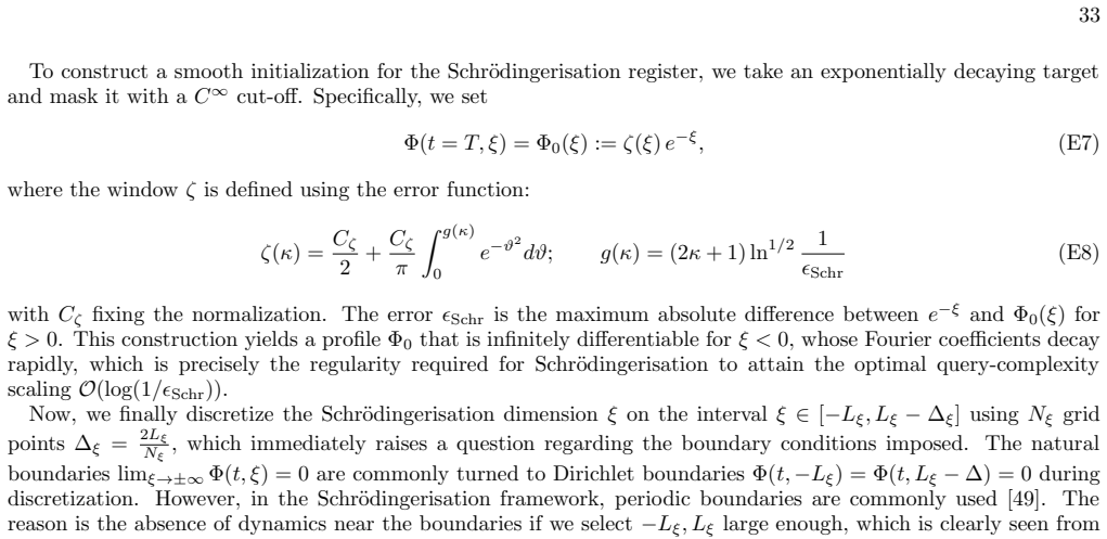
The construction of the initial state and the smooth cut-off for Schr¨ odingerisation are given in Appendix F
End-to-end complexity scaling We now collect the dominant gate complexities of the one-asset Heston pipeline for estimating a single option value V (0, S0, v0). The construction of the initial state and the smooth cut-off for Schr¨ odingerisation are given in Appendix F. The auxiliary register size nξ and the resulting non-conservative evolution are discu...
-
[6]
(D12), we perform the same method-of-lines reduction as in Appendix B.2
Linear ODE system for Multi-asset Heston model Starting from the continuous multi-asset Heston PDE in Eq. (D12), we perform the same method-of-lines reduction as in Appendix B.2. Consider d underlying assets with prices S = (S1, . . . , Sd) and variance variablesv = (v1, . . . , vd), and let V (t, S, v) denote the option value. We discretize each coordina...
-
[7]
As in Appendix B.3, the total cost is the sum of state preparation and backward evolution, multiplied by the single-point readout overhead
End-to-end complexity scaling We summarize the dominant end-to-end cost for the multi-asset Heston model (D12). As in Appendix B.3, the total cost is the sum of state preparation and backward evolution, multiplied by the single-point readout overhead. For this estimate, we use the Worst-of Call payoff in Eq. (D13). The main difference from the multi-asset...
-
[8]
(E16) inside the quantum device
Block-encoding as an input model In this subsection we address an important problem on how to input the model Hamiltonian H = −Xη ⊗ S1 + Iη ⊗ S2. (E16) inside the quantum device. We focus on the block-encoding technique as it is known how to implement it on gate level efficiently [14, 15]. Block-encoding technique incorporates a non-unitary matrix of inte...
-
[9]
O(dQσn log n + nξ log nξ + dηsn) quantum gates,
-
[10]
The Qσ parameter describes the maximum degree of the polynomial approximation for the local volatility σi(Si) ≈PQσ−1 k=0 κkSk i (can be generalized to piecewise local vol)
O(n) ancilla qubits. The Qσ parameter describes the maximum degree of the polynomial approximation for the local volatility σi(Si) ≈PQσ−1 k=0 κkSk i (can be generalized to piecewise local vol). The parameter η ∼ d2 is the number of terms in the original PDE. We highlight that in Proposition 3 the resulting block-encoding UH constant α necessarily contains...
-
[11]
The key technique here is called Alternating phase modulation sequence which allows one to polynomially transform the matrix under block-encoding
Evolution operator implementation In this subsection we consider how several block-encodings UH (or conjugated version U † H ) can be used to imple- ment the evolution operator eiHt. The key technique here is called Alternating phase modulation sequence which allows one to polynomially transform the matrix under block-encoding. Definition 2 (Alternating p...
-
[12]
Pq(x) has parity (0 or 1 mod 2) , which means that it has only odd or even degrees of x
-
[13]
Pq(x) is a real polynomial, which means that all the coefficients are real
-
[14]
36 𝑈 𝐻 𝑑𝑛 + 𝑛 𝜉 + 1 𝑈 Φ = 𝑈 𝐻 𝑈 𝐻 … 𝐶 𝜙 1 0 … 0 𝑞 - �mes † 𝑠 𝐶 𝜙 2 0 … 0 𝐶 𝜙 𝑞 0 … 0 Fig
For all x ∈ [−1, 1]: |Pq(x)| < 1. 36 𝑈 𝐻 𝑑𝑛 + 𝑛 𝜉 + 1 𝑈 Φ = 𝑈 𝐻 𝑈 𝐻 … 𝐶 𝜙 1 0 … 0 𝑞 - �mes † 𝑠 𝐶 𝜙 2 0 … 0 𝐶 𝜙 𝑞 0 … 0 Fig. 9: A schematic circuit view for the Alternating phase transformation sequence (for odd polynomial degree q). The phase gate C00...0 ϕ is given by (E25). The circuit allows to implement a block-encoding of a polynomial poly(H) which o...
-
[15]
Recovery of the ODE solution After Proposition 5 we return to the solution of the original system (E1). The Schr¨ odingerisation procedure embeds the dynamics into a register decomposed (from left to right) as c|{z} evol ancillas , W + 1| {z } system , n ξ|{z} Schr¨ odingerisation , a prep|{z} prep ancillas , (E29) so that c qubits are used as block-encod...
-
[16]
O (Qmaxn log n + Gn + QmaxG) C-NOT and single-qubit gates,
-
[17]
with success probability proportional to the filling ratio F := ∥f ∥2 2/(2∥f ∥2 max)
n − 1 ancilla qubits. with success probability proportional to the filling ratio F := ∥f ∥2 2/(2∥f ∥2 max). (F2) The probability of success psuccess = O(F) in Proposition 6 can be further boosted using the method described in Appendix J. Thus, one can implement ( O(1), c, ϵevol) using ≈ 1/ √ F queries to Uf and U † f. The vanilla option payoff max(0 , S −...
-
[18]
Basket option payoffs To implement the basket option payoffs from Table V, we rely on the main technique underlying Proposition 6, often referred to as the indicator qubit method [48]. In this approach, we reversibly (i.e., via a unitary operation) set an auxiliary qubit to the state |1⟩ on a chosen region of interest: ∀ |ψ⟩ = 2n−1X i=0 ψi |i⟩ , U k indic...
-
[19]
|0⟩aprep ⟨0|aprep with aprep = d⌈log2 n⌉ + 3d arising from the quantum state preparation (Proposition 6)
-
[20]
|0⟩c ⟨0|c with c = d⌈log2 n⌉ + ⌈log2 nξ⌉ + ⌈log2 s⌉ + ⌈log2 η⌉ + 4d + 7 coming from the evolution stage (Proposi- tion 5), where d → 2d for the Heston model
-
[21]
Π ξ>0 =P2nξ −1 k=kλ |k⟩nξ ⟨k|nξ with kλ = ⌈λmin S1 /∆ξ⌉ induced by Schr¨ odingerisation (see Eq. (E5)). The state |ς⟩a indicates a successful projection to the subspace generated by the Π and up to O(log 1 ϵSchr ) has the form: |ς⟩a = |0⟩aprep ⊗ |0⟩c ⊗ 1qP2nξ −1 m=kλ e−2m∆ξ 2nξ −1X k=kλ e−k∆ξ |k⟩nξ . (G2) We note that this state is easy to prepare using P...
-
[22]
Single amplitude estimation In this subsection we provide an algorithm on how to estimate a fixed coefficient ψq of the pricing state |ψ⟩W =P2W −1 i=0 ψi |i⟩W . We recall that the block-encoding U satisfies (Π ⊗ I ⊗W )U |0⟩W+a = Nς |ς⟩a ⊗ |ψ⟩W , (G4) where Nς = O(1) is assumed known (computed from the Sections E, F) and |ς⟩a lies in the image of Π. Next, ...
-
[23]
In this paper we use this normalization factor to find the option values using Eq
Normalization factor propagation Let us now address the problem of finding NV (t) = r P i V (t, ⃗Si, ⃗ vi) 2 for 0 ≤ t ≤ T . In this paper we use this normalization factor to find the option values using Eq. (G3). Proposition 7 allows us to find ψq; which together with NV (t = 0) allows us to find the option prices. 42 We first remind the reader that the ...
-
[24]
One of them is to directly record the number of successful postselections in the nξ-qubit register from the quantum scheme in Fig. 1. Denoting by ˆ p the empirical success probability, the corresponding Monte-Carlo (shot-noise) scaling is Nshots = O 1 ϵ2 shot log 1 δ , ϵ shot := |ˆp − Pr ξ > λ min S1 | Pr ξ > λ min S1 . (G22) The given dependence is not o...
-
[25]
The resulting error scaling is Nshots = O 1 ϵshot log 1 δ , (G23) which is an optimal scaling
Another way is to use Proposition 7 with the whole quantum circuit as an observable A. The resulting error scaling is Nshots = O 1 ϵshot log 1 δ , (G23) which is an optimal scaling. Finally, the normalization factor NV (t = 0) is estimated by rearranging Eq. (G21) as NV (t = 0) = NV (t = T ) s Pr ξ > λ min S1 CλS . (G24) Consequently, if bNV (t = T ) has ...
-
[26]
(G1) is necessary to estimate the single value V (t = 0, ⃗Sq, ⃗ vq) with error ϵV
Complexity scaling for readout Now, we estimate how many applications of U from Eq. (G1) is necessary to estimate the single value V (t = 0, ⃗Sq, ⃗ vq) with error ϵV . Fix a target grid point q corresponding to ( ⃗Sq, ⃗ vq). The readout step is V (t = 0, ⃗Sq, ⃗ vq) = ψq NV (t = 0). (G26) As in the Hadamard-test construction, we estimate ψq via mIQAE appli...
-
[27]
Now we introduce complexity analysis for SDE Monte Carlo methods
SDE-based Monte Carlo baselines The estimates above are grid-based PDE estimates. Now we introduce complexity analysis for SDE Monte Carlo methods. This is a different classical benchmark. A PDE method discretizes the state space, while an SDE Monte Carlo method simulates paths and averages the resulting payoffs. Thus the full N d spatial grid does not ap...
-
[28]
Brownian corr
shown in Table IX. Brownian corr. structure Cost per Brownian step Cost in ε Cost using ε ≍ 2−2n Dense correlation O(d2) O(d2ε−2) O(d224n) q-factor correlation O(dq) O(dq ε−2) O(dq 24n) Diagonal correlation O(d) O(dε−2) O(d 24n) Table IX: Multivariate Black–Scholes case: Monte Carlo complexity when the terminal lognormal distribution is sampled exactly. T...
-
[29]
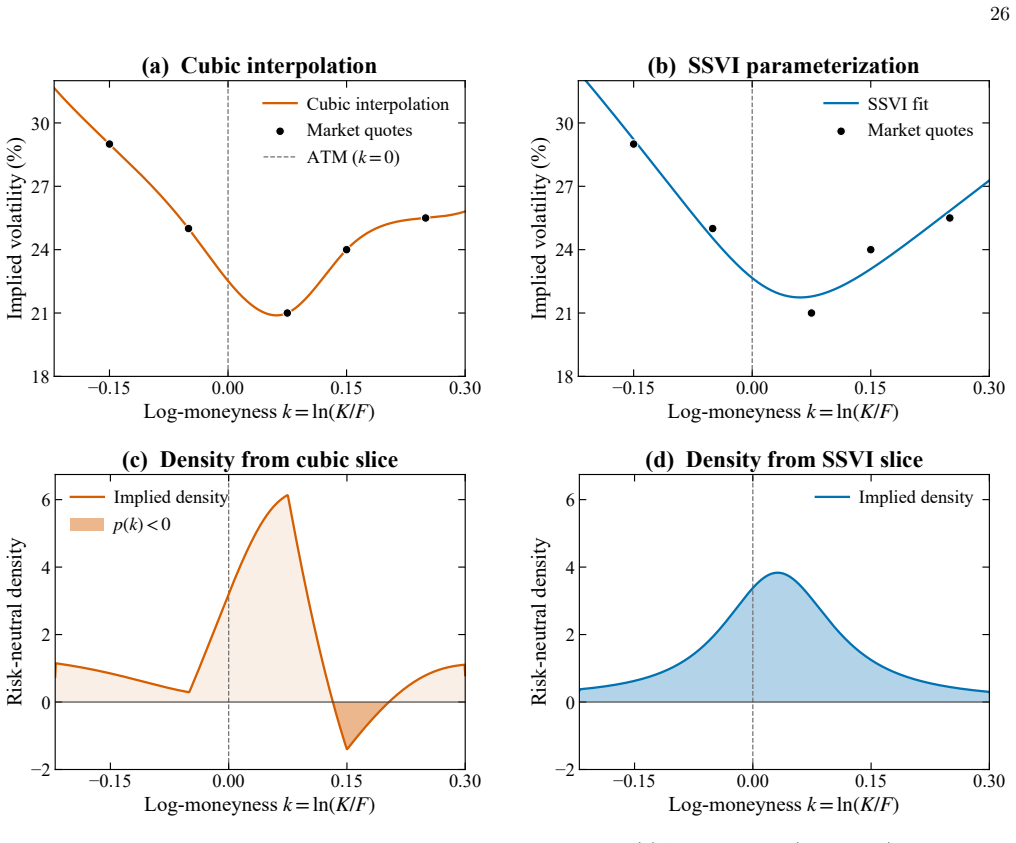
We write N and ϕ for the standard normal CDF and pdf: N(x) = Z x −∞ 1√ 2π e−u2/2 du, ϕ (x) = 1√ 2π e−x2/2
Durrleman’s g–function and butterfly arbitrage To make the butterfly-arbitrage check explicit, we recall the standard Durrleman / Gatheral–Jacquier factorization for a single implied-volatility slice. We write N and ϕ for the standard normal CDF and pdf: N(x) = Z x −∞ 1√ 2π e−u2/2 du, ϕ (x) = 1√ 2π e−x2/2. (K4) Use ϕ for the standard normal density and re...
discussion (0)
Sign in with ORCID, Apple, or X to comment. Anyone can read and Pith papers without signing in.