pith. sign in

arxiv: 2605.27126 · v1 · pith:WWIP5YLRnew · submitted 2026-05-26 · 🧮 math.GT · math.SG

A contact version of Kirby's theorem

Pith reviewed 2026-06-29 14:30 UTC · model grok-4.3

classification 🧮 math.GT math.SG
keywords contact surgeryKirby movescontact 3-manifoldsLegendrian linkslantern movechain movefront projection
0
0 comments X

The pith

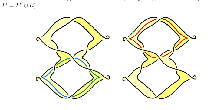
Two contact surgery diagrams represent contactomorphic 3-manifolds precisely when connected by planar isotopies, Legendrian Reidemeister moves, cancelling pairs, handle slides, lantern moves, and chain moves.

A machine-rendered reading of the paper's core claim, the machinery that carries it, and where it could break.

The paper establishes a complete set of diagrammatic moves for contact surgery presentations of closed connected contact 3-manifolds. Every such manifold arises by contact (±1)-surgery on a Legendrian link in the standard tight sphere, but earlier operations like cancelling pairs and handle slides alone fail to relate all equivalent diagrams. The authors add the lantern move and chain move to the list and prove that the full collection of eight operations generates every equivalence. A sympathetic reader would care because the result supplies an explicit front-projection calculus that lets one manipulate diagrams directly to decide whether two presentations describe the same contact structure.

Core claim

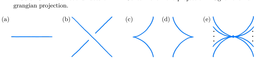
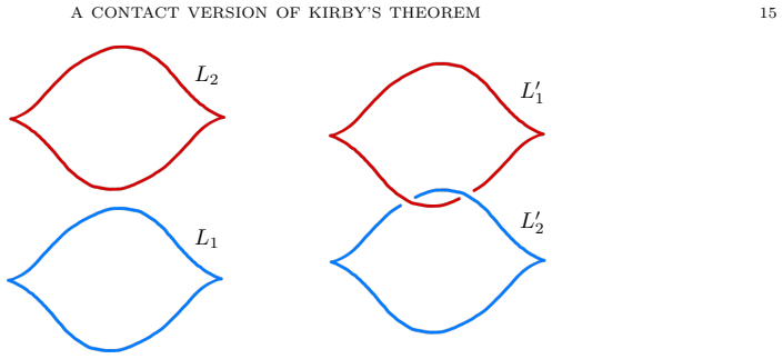
Two contact surgery diagrams represent contactomorphic contact manifolds if and only if they are related by a sequence of planar isotopies, Legendrian Reidemeister moves, insertions or removals of standard cancelling pairs, the two standard contact handle slides, the standard lantern move, and the standard chain move. All these moves are explicit diagrammatic operations in the front projection.

What carries the argument

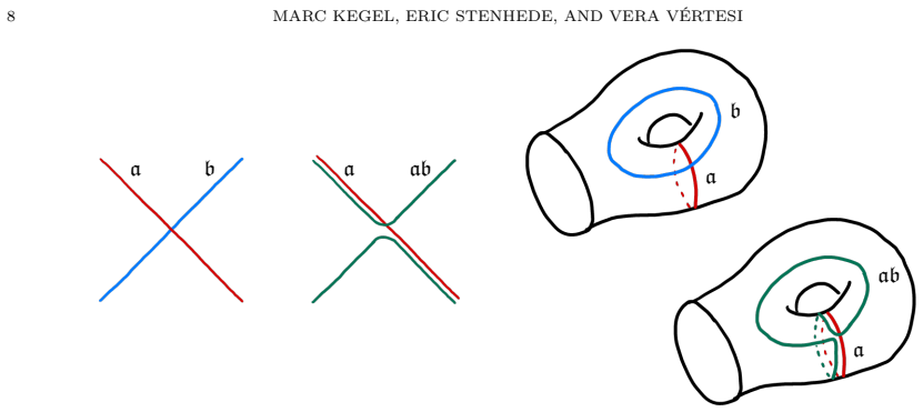
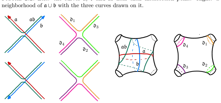
The standard lantern move and standard chain move, which complete the set of contact Kirby moves when combined with isotopies, Reidemeister moves, cancelling pairs, and handle slides via the ribbon-move framework.

If this is right

  • Gompf's d3-invariant is unchanged by each of the eight moves and can be recovered directly from the diagram without reference to the manifold.
  • The classical topological Kirby theorem follows as a corollary obtained by forgetting the contact structure.
  • Any two contact surgery diagrams of the same manifold can be transformed into each other using only these front-projection operations.
  • The moves give a practical method for comparing contact structures by reducing one diagram to the other.

Where Pith is reading between the lines

These are editorial extensions of the paper, not claims the author makes directly.

  • The calculus could be applied to decide contactomorphism by attempting to reduce both diagrams to a common normal form.
  • Similar diagrammatic presentations might be sought for contact structures in higher dimensions or for other geometric structures on 3-manifolds.
  • Contact-geometric techniques may yield new proofs of purely topological results beyond the Kirby theorem.

Load-bearing premise

Avdek's ribbon-move framework together with Gervais' presentation of the mapping class group generates all equivalences that arise from contactomorphisms of the surgered manifolds.

What would settle it

Two diagrams of contactomorphic manifolds whose front projections cannot be connected by any finite sequence of the eight listed moves.

Figures

Figures reproduced from arXiv: 2605.27126 by Eric Stenhede, Marc Kegel, Vera V\'ertesi.

Figure 1.1
Figure 1.1. Figure 1.1: A standard cancelling pair. ↔ ↔ − − − − − − − − [PITH_FULL_IMAGE:figures/full_fig_p002_1_1.png] view at source ↗
Figure 1.2
Figure 1.2. Figure 1.2: The two standard contact handle slides needed in Theorem 1.1. − − − − − − ↔ − [PITH_FULL_IMAGE:figures/full_fig_p002_1_2.png] view at source ↗
Figure 1.3
Figure 1.3. Figure 1.3: The standard lantern move. 1.1. The standard contact Kirby moves. We now describe the standard contact Kirby moves appearing in Theorem 1.1. In Section 11 we verify that these moves do not change the contactomorphism type of the surgered contact manifolds. In Figures 1.1–1.4, the shaded region indicates the front projection of the supporting surface or handlebody on which the move is performed. The corre… view at source ↗
Figure 1.4
Figure 1.4. Figure 1.4: The standard chain move. • The standard chain move is the move shown in [PITH_FULL_IMAGE:figures/full_fig_p003_1_4.png] view at source ↗
Figure 2.1
Figure 2.1. Figure 2.1: The curves a, b and ab near the intersection point a ∩ b. If a and b intersect transversely at a single point, then ab is isotopic to τ + a (b). Example 2.3 (Braid relations). Let a and b be simple closed curves intersecting transversely at a single point. Then τ + a τ + b = τ + ab τ + a . This is a braid relation; see [PITH_FULL_IMAGE:figures/full_fig_p007_2_1.png] view at source ↗
Figure 2.2
Figure 2.2. Figure 2.2: Left: the curves a, b and ab near their intersection point. Right: a neighborhood of a ∪ b with the three curves drawn on it. a b ab d1 d3 d2 d4 ab b a d4 d3 d1 d2 [PITH_FULL_IMAGE:figures/full_fig_p008_2_2.png] view at source ↗
Figure 2.3
Figure 2.3. Figure 2.3: Left: the curves in a lantern relation near the two intersection points of a and b (which have opposite sign). Right: a neighborhood of a ∪ b with all the curves drawn. Example 2.5 (Chain relations). Let a, b and c be simple closed curves such that a and b intersect transversely in one point, b and c intersect transversely in one point, and a ∩ c = ∅. Then [PITH_FULL_IMAGE:figures/full_fig_p008_2_3.png] view at source ↗
Figure 2.4
Figure 2.4. Figure 2.4: Left: the curves in a chain relation near the intersection points of a with b and of b with c. Right: a neighborhood of a ∪ b ∪ c with the curves a, b,c, d1, d2 drawn [PITH_FULL_IMAGE:figures/full_fig_p008_2_4.png] view at source ↗
Figure 3.1
Figure 3.1. Figure 3.1: Left: coordinates on R 3 . Center: the front projection. Right: the La￾grangian projection. (a) (b) (c) (d) (e) · · · · · · [PITH_FULL_IMAGE:figures/full_fig_p010_3_1.png] view at source ↗
Figure 3.2
Figure 3.2. Figure 3.2: Local models for points in the front projection of a generic Legendrian graph. in the (x, y)–plane. Once rL and the value of the z–coordinate at one point r(s0) are known, the full Legendrian curve can be reconstructed from the formula rz(s) = rz(s0) − Z s s0 rx(u) r ′ y (u) du. In particular, if r is closed, then I rL x dy = 0. Furthermore, r is embedded precisely when every loop in the Lagrangian proje… view at source ↗
Figure 3.3
Figure 3.3. Figure 3.3: Lagrangian projections corresponding to the front projections in Fig￾ure 3.2. The y–coordinate agrees with that of the front projection, and the x–coordinate parametrizes the vertical direction (top to bottom is positive). The following two Reidemeister theorems for Legendrian links and Legendrian graphs were first shown in [Swi92] and [BI09, Proposition 4.2]. Theorem 3.1 (Swiatkowski [Swi92]). Two Legen… view at source ↗
Figure 3.4
Figure 3.4. Figure 3.4: Legendrian Reidemeister moves for Legendrian links. Horizontal and vertical reflections of these moves are also allowed, with crossings adjusted appropriately. No other Legendrian strand of the diagram is allowed to appear in these pictures. ←−→ IIG R ←→ · · · · · · [PITH_FULL_IMAGE:figures/full_fig_p011_3_4.png] view at source ↗
Figure 3.5
Figure 3.5. Figure 3.5: Additional Legendrian Reidemeister moves for Legendrian graphs. Hori￾zontal and vertical reflections of these moves are again allowed. 4. Convex surfaces Let Σ be an oriented surface embedded in a contact manifold (M, ξ). We denote by Σξ the characteristic foliation induced on Σ. The surface Σ is called convex if there exists a contact vector field X which is everywhere transverse to Σ. An equivalent for… view at source ↗
Figure 7.1
Figure 7.1. Figure 7.1: Left: a Legendrian graph G. Right: a ribbon surface R of G. For L, we can embed L1 in a perturbation of R × {t1} and L2 in a perturbation of R × {t2} with t2 > t1, as illustrated in [PITH_FULL_IMAGE:figures/full_fig_p014_7_1.png] view at source ↗
Figure 7.2
Figure 7.2. Figure 7.2: Left: a Legendrian link L = L1 ∪ L2. Right: another Legendrian link L ′ = L ′ 1 ∪ L ′ 2 [PITH_FULL_IMAGE:figures/full_fig_p015_7_2.png] view at source ↗
Figure 7.3
Figure 7.3. Figure 7.3: Left: L1 embedded in R × {t1}. Right: L2 embedded in R × {t2} with t2 > t1. Before we discuss the next lemma, we need a definition. Given a Legendrian graph G whose vertices all have valency 4 and whose front projections look as on the left of [PITH_FULL_IMAGE:figures/full_fig_p015_7_3.png] view at source ↗
Figure 7.4
Figure 7.4. Figure 7.4: Left: the local model around a generic valency 4 vertex v. Right: the two possible resolutions of v. Lemma 7.9. Let G be a Legendrian graph whose vertices all have valency 4 and look as in [PITH_FULL_IMAGE:figures/full_fig_p015_7_4.png] view at source ↗
Figure 7.5
Figure 7.5. Figure 7.5: Left: Lagrangian projection of a neighborhood in Re of a vertex of G. Right: Lagrangian projections of the two possible resolutions [PITH_FULL_IMAGE:figures/full_fig_p015_7_5.png] view at source ↗
Figure 7.6
Figure 7.6. Figure 7.6: Top: front projections of a valency 4 vertex before and after a Reidemeister move R. Bottom: corresponding Lagrangian projections. Corollary 7.11. Any resolution of a Legendrian graph G whose vertices have valency 4 is embedded in a perturbation of any ribbon surface of G. Proof. By definition, G is contained in any ribbon surface R of itself. The claim follows from Lemma 7.9. □ Another useful lemma that… view at source ↗
Figure 8.1
Figure 8.1. Figure 8.1: Left: a ribbon surface Σ. Middle: the product Σ × [−ε, ε]. Right: a regular neighborhood H of G equipped with a half open book structure [PITH_FULL_IMAGE:figures/full_fig_p017_8_1.png] view at source ↗
Figure 8.2
Figure 8.2. Figure 8.2: Left: a ribbon surface R. Right: the product R × [−ε, ε], viewed as a neighborhood of the Legendrian graph. By rounding the edges of U, we obtain a standard regular neighborhood H of G, which can be seen as H ∼= Σ × [−ε, ε]/∼, [PITH_FULL_IMAGE:figures/full_fig_p017_8_2.png] view at source ↗
Figure 10.1
Figure 10.1. Figure 10.1: Left: the contact surgery link L = L − 1 ∪ L − 2 . Right: the contact surgery link L ′ = L ′− 1 ∪ L ′− 2 . Lemma 10.3. Let L and L ′ be two RG–equivalent contact surgery links. Then L and L ′ are also RG′–equivalent for every Legendrian graph G′ containing G. Proof. By Lemma 7.12, L and L ′ are both compatible with RG′ . Moreover, viewing RG as a subsurface of RG′ , any diffeomorphism of RG fixing ∂RG e… view at source ↗
Figure 10.2
Figure 10.2. Figure 10.2: Left: the contact surgery link L = L − 1 ∪ L − 2 ∪ K+. Right: the contact surgery link L ′ = L ′− 1 ∪ L ′− 2 ∪ K+. The point of introducing ribbon moves is the following result. Proposition 10.7 ([Avd13, Proposition 6.3]). Suppose that a contact surgery link L in (S 3 , ξst) can be transformed into another contact surgery link L ′ by a sequence of ribbon moves. Then L and L ′ describe contactomorphic co… view at source ↗
Figure 11.1
Figure 11.1. Figure 11.1: Left: a Legendrian graph G which is a copy of either component of [PITH_FULL_IMAGE:figures/full_fig_p020_11_1.png] view at source ↗
Figure 11.2
Figure 11.2. Figure 11.2: Left: the contact surgery link L = L − 1 ∪ L − 2 . Right: the contact surgery link L ′ = L ′− 1 ∪ L ′− 2 . G R [PITH_FULL_IMAGE:figures/full_fig_p021_11_2.png] view at source ↗
Figure 11.3
Figure 11.3. Figure 11.3: Left: the Legendrian graph G underlying the braid relation. Right: a ribbon surface R of G. − − − − [PITH_FULL_IMAGE:figures/full_fig_p021_11_3.png] view at source ↗
Figure 11.4
Figure 11.4. Figure 11.4: Another pair of contact surgery links differing by an elementary R–equivalence corresponding to a braid relation. 11.3. Lantern relation. Let L = L − 1 ∪ L − 2 ∪ L − 3 be a contact surgery link. Suppose that there are two balls in which L looks as in the left column of [PITH_FULL_IMAGE:figures/full_fig_p021_11_4.png] view at source ↗
Figure 11.5
Figure 11.5. Figure 11.5: Left: the contact surgery link L = L − 1 ∪ L − 2 ∪ L − 3 . Right: the contact surgery link L ′ = L ′− 1 ∪ L ′− 2 ∪ L ′− 3 ∪ L ′− 4 produced by a lantern move [PITH_FULL_IMAGE:figures/full_fig_p022_11_5.png] view at source ↗
Figure 11.6
Figure 11.6. Figure 11.6: A ribbon surface R compatible with the contact surgery links appearing in the lantern move. 11.4. Chain relation. We consider the contact surgery links L = [ 12 i=1 L − i , L ′ = L ′− 1 ∪ L ′− 2 whose local pictures are as in [PITH_FULL_IMAGE:figures/full_fig_p022_11_6.png] view at source ↗
Figure 11.7
Figure 11.7. Figure 11.7: Left: the contact surgery link L = S12 i=1 L − i . Right: the contact surgery link L ′ = L ′− 1 ∪ L ′− 2 [PITH_FULL_IMAGE:figures/full_fig_p023_11_7.png] view at source ↗
Figure 11.8
Figure 11.8. Figure 11.8: A ribbon surface R compatible with the contact surgery links appearing in the chain move. where we use Regina’s notation. Since all contact surgery coefficients in these local diagrams are equal to (−1), the resulting contact structures are Stein fillable, and hence tight. Using [LS07b; LM04], one checks that both M1 and M2 are L-spaces. The tight contact structures on these Seifert fibered spaces were … view at source ↗
Figure 11.9
Figure 11.9. Figure 11.9: Left: local model of an intersection between successive knots in the chain. The ribbon surface R is also shown here. Right: local pictures of L (first column) and L ′ (second column) near a vertex; top row for intersections between K2k and K2k+1, bottom row for intersections between K2k−1 and K2k for k = 1, . . . , n. p p [PITH_FULL_IMAGE:figures/full_fig_p024_11_9.png] view at source ↗
Figure 11.10
Figure 11.10. Figure 11.10: Legendrian isotopy of L near the intersection between K1 and K2: the point p travels around K1. p p [PITH_FULL_IMAGE:figures/full_fig_p024_11_10.png] view at source ↗
Figure 11.11
Figure 11.11. Figure 11.11: Legendrian isotopy near the intersection between K2n and K2n+1. p q q p [PITH_FULL_IMAGE:figures/full_fig_p024_11_11.png] view at source ↗
Figure 11.12
Figure 11.12. Figure 11.12: Legendrian isotopy near consecutive intersections between K2k, K2k+1 and K2k+1, K2k+2: the intersection points p and q slide along K2k+1 [PITH_FULL_IMAGE:figures/full_fig_p024_11_12.png] view at source ↗
Figure 12.1
Figure 12.1. Figure 12.1: The surface Σ bounded by a∪b and the chain Ge (in purple) whose regular neighborhood is Σ. 13. Proof of the contact Kirby theorem In this section, we prove Theorem 1.1. The main ingredients have already been established: Avdek’s theorem reduces the problem to ribbon moves, and the preceding sections identify the elementary R￾equivalences that are needed. We now explain how these ribbon moves translate i… view at source ↗
Figure 13.1
Figure 13.1. Figure 13.1: The box labelled G on the left symbolizes the Legendrian graph G. We are attaching to G (using a Legendrian arc) the purple Legendrian graph on the right of this figure. some contact surgery link compatible with Re. Thus, we obtain a sequence of contact surgery links L = L 0 , L 1 , . . . , L k = L ′ such that • each L i is compatible with Re; • the mapping class of L i is the one obtained from τL after… view at source ↗
Figure 13.2
Figure 13.2. Figure 13.2: Legendrian graphs Gchain and Glantern whose ribbons support the standard chain and lantern relations. 14. A toolbox of contact Kirby moves In this section, we collect contact Kirby moves from the literature, their diagrammatic representatives, and the new moves introduced in this article. The section is intended as a ready-to-use toolbox for readers who want to manipulate contact surgery diagrams withou… view at source ↗
Figure 14.1
Figure 14.1. Figure 14.1: Contact handle slides. The blue component may be unframed; if it is a surgery component, its surgery coefficient is preserved. 14.4. Lantern destabilizations. Lantern destabilizations were introduced by Lisca and Stipsicz [LS11]. They form a family of contact Kirby moves, indexed by the number of additional strands passing through the picture. Their proof proceeds by translating from the relevant surger… view at source ↗
Figure 14.2
Figure 14.2. Figure 14.2: Further contact handle slides. Again, the blue component may be unframed; if it is a surgery component, its surgery coefficient is preserved. + − }± }k + }± }k [PITH_FULL_IMAGE:figures/full_fig_p030_14_2.png] view at source ↗
Figure 14.3
Figure 14.3. Figure 14.3: The lantern destabilizations with k ∈ Z≥0 strands, shown in grey. 14.5. Lantern and chain moves. The lantern and chain moves considered in this article arise from the corresponding lantern and chain relations in the mapping class group. They are constructed in Section 11 by translating these mapping class group relations into contact surgery diagrams using compatible ribbon surfaces and open books. Spec… view at source ↗
Figure 14.4
Figure 14.4. Figure 14.4: Two examples of lantern moves. All components are decorated with a − sign. 14.6. Other moves in the literature. There are other contact Kirby moves in the literature. Examples include the contact annulus twist of [CEK24] and various contact Rolfsen twists [DG09; Keg18; Keg17; KO23]. These are useful operations in their own right. However, for the purposes of this paper, we do [PITH_FULL_IMAGE:figures/f… view at source ↗
Figure 14.5
Figure 14.5. Figure 14.5: Two further examples of lantern moves. All components are decorated with a − sign [PITH_FULL_IMAGE:figures/full_fig_p031_14_5.png] view at source ↗
Figure 14.6
Figure 14.6. Figure 14.6: Two more examples of lantern moves arising from the lantern relation. All components are decorated with a − sign [PITH_FULL_IMAGE:figures/full_fig_p031_14_6.png] view at source ↗
Figure 14.7
Figure 14.7. Figure 14.7: Two examples of chain moves. All components are decorated with a − sign [PITH_FULL_IMAGE:figures/full_fig_p031_14_7.png] view at source ↗
Figure 14.8
Figure 14.8. Figure 14.8: Two further examples of chain moves. All components are decorated with a − sign [PITH_FULL_IMAGE:figures/full_fig_p031_14_8.png] view at source ↗
Figure 14.9
Figure 14.9. Figure 14.9: Two more examples of chain moves. All components are decorated with a − sign [PITH_FULL_IMAGE:figures/full_fig_p032_14_9.png] view at source ↗
Figure 14.10
Figure 14.10. Figure 14.10: Additional examples of chain moves; again all components have coefficient −. not include them as basic moves in the toolbox below since the contact annulus twist can be expressed as an explicit sequence of contact handle slides followed by a cancellation [CEK24], while contact Rolfsen twists can be explicitly expressed in terms of contact handle slides and lantern destabilizations [KO23]. 15. Homotopic… view at source ↗
Figure 15.1
Figure 15.1. Figure 15.1: The oriented standard lantern move. The labels and orientations determine the matrices A, A′ and the rotation vectors a, a ′ . The left and right parts of L2 and L3 are the parts of these knots on the left and on the right of the dotted line. Standard chain move. Finally, we consider the standard chain move along the oriented link illustrated in [PITH_FULL_IMAGE:figures/full_fig_p035_15_1.png] view at source ↗
Figure 15.2
Figure 15.2. Figure 15.2: The oriented standard chain move. Only the components L1, L2, and L3 are labelled explicitly. The remaining components are labelled by moving upwards through the diagram: L4 is the second green unknot, L5 is the second blue unknot, and so on, ending with L12, the highest red unknot. σ(Q ′ ) − σ(Q) = σ(A ′ ) − σ(A). In particular, it follows that if (a ′ ) T (A ′ ) −1a ′ − a T A −1a = 3 σ(A ′ ) − σ(A)  … view at source ↗
Figure 16.1
Figure 16.1. Figure 16.1: A contact handle slide expressed as the insertion of a standard cancelling pair, a standard contact handle slide, and the removal of a standard cancelling pair. Set ab = τ + a (b). Then τ + a τ − b = τ − abτ + abτ + a τ − b = τ − ab τ + abτ + a  τ − b = τ − ab τ + a τ + b  τ − b by the braid relation, applied backwards = τ − abτ + a [PITH_FULL_IMAGE:figures/full_fig_p039_16_1.png] view at source ↗
Figure 16.2
Figure 16.2. Figure 16.2: Steps (1)–(4) in the proof of the lantern destabilization: the initial diagram, a Legendrian isotopy, the insertion of one standard cancelling pair, and the insertion of two further standard cancelling pairs. Figures 16.2–16.5 give a diagrammatic realization of this transformation using only the allowed moves. More precisely, [PITH_FULL_IMAGE:figures/full_fig_p040_16_2.png] view at source ↗
Figure 16.3
Figure 16.3. Figure 16.3: Steps (5)–(8): a lantern move, the removal of a standard cancelling pair, and Legendrian isotopies of the purple and red components [PITH_FULL_IMAGE:figures/full_fig_p040_16_3.png] view at source ↗
Figure 16.4
Figure 16.4. Figure 16.4: Steps (9)–(12): Legendrian isotopies of the pink component, followed by a contact handle slide and the removal of a standard cancelling pair involving the red and pink components. + +− + [PITH_FULL_IMAGE:figures/full_fig_p041_16_4.png] view at source ↗
Figure 16.5
Figure 16.5. Figure 16.5: Steps (13)–(14): a Legendrian isotopy of the purple component, followed by a contact handle slide and the removal of a standard cancelling pair involving the blue and purple components. 17. Legendrian knots in contact surgery diagrams Here we prove the contact version of Kirby’s theorem for Legendrian links presented in contact surgery diagrams. Proof of Theorem 1.6. Let Ji be a Legendrian link in a con… view at source ↗
Figure 17.1
Figure 17.1. Figure 17.1: Removing intersections of the black curve with the shaded region by handle slides. The case of the chain move is slightly more involved. In the middle of [PITH_FULL_IMAGE:figures/full_fig_p042_17_1.png] view at source ↗
Figure 17.2
Figure 17.2. Figure 17.2: Removing intersections of the black curve with the shaded region by handle slides. In [PITH_FULL_IMAGE:figures/full_fig_p042_17_2.png] view at source ↗
Figure 17.3
Figure 17.3. Figure 17.3: An isotopy of the red curve in the complement of the orange and purple curves. 18. Blow-ups and blow-downs in contact geometry We now make precise the heuristic mentioned in Remark 1.8. Let M = H1 ∪h H2 be a Heegaard splitting with Heegaard surface Σ = ∂H1 = ∂H2. If a mapping class g ∈ MCG(Σ) extends over the handlebody H1, then replacing the gluing map h by h ◦ g −1 gives the same 3-manifold. Indeed, t… view at source ↗
read the original abstract

A theorem of Ding and Geiges states that every closed, connected contact $3$-manifold can be obtained from the standard tight contact $3$-sphere by contact $(\pm1)$-surgery along a Legendrian link. The literature also contains some examples of contact Kirby moves, i.e. explicit operations on front projections of Legendrian surgery links that change the surgery link but preserve the contactomorphism type of the surgered manifold. Among the most commonly used are cancelling pairs and contact handle slides; however, these moves alone are not sufficient to relate all contact surgery diagrams of contactomorphic contact manifolds. In this article, we introduce two new families of contact Kirby moves, called lantern moves and chain moves, and use them to give a complete set of contact Kirby moves. More precisely, we show that two contact surgery diagrams represent contactomorphic contact manifolds if and only if they are related by a sequence of planar isotopies, Legendrian Reidemeister moves, insertions or removals of standard cancelling pairs, the two standard contact handle slides, the standard lantern move, and the standard chain move. All these moves are explicit diagrammatic operations in the front projection. The proof follows an approach initiated by Avdek through his ribbon-move framework, which is rooted in the Giroux correspondence, and combines it with a presentation by Gervais of the mapping class group. We also discuss several consequences of the main theorem, illustrating the effectiveness of the contact Kirby calculus by recovering the invariance of Gompf's $d_3$-invariant purely diagrammatically and by deriving the topological Kirby theorem from contact-geometric methods.

Editorial analysis

A structured set of objections, weighed in public.

Desk editor's note, referee report, simulated authors' rebuttal, and a circularity audit. Tearing a paper down is the easy half of reading it; the pith above is the substance, this is the friction.

Referee Report

2 major / 2 minor

Summary. The paper claims to establish a complete contact-geometric analogue of Kirby's theorem: two contact surgery diagrams on Legendrian links in the standard tight contact 3-sphere represent contactomorphic contact 3-manifolds if and only if they are related by planar isotopies, Legendrian Reidemeister moves, insertions or removals of standard cancelling pairs, the two standard contact handle slides, the standard lantern move, and the standard chain move. All moves are explicit in the front projection. The proof combines Avdek's ribbon-move framework (via the Giroux correspondence) with Gervais' finite presentation of the mapping class group; consequences include a purely diagrammatic proof of the invariance of Gompf's d_3-invariant and a contact-geometric derivation of the classical topological Kirby theorem.

Significance. If the central claim holds, the result supplies a practical, fully explicit diagrammatic calculus for contact surgery, a foundational operation in contact topology. The explicit front-projection moves and the recovery of d_3-invariance directly from the moves constitute concrete strengths; likewise, deriving the topological Kirby theorem from contact-geometric methods illustrates the framework's reach. The work builds on existing tools (Avdek, Gervais, Giroux) to produce a usable move set rather than an existence result.

major comments (2)
  1. [Proof of the main theorem] Main theorem (proof section combining Avdek ribbon moves with Gervais MCG presentation): the completeness of the listed move set rests on the assertion that the lantern move, chain move, and classical operations realize every generator and relation in Gervais' presentation when transported through Avdek's framework. The manuscript does not supply an explicit enumeration, table, or case-by-case verification showing how each MCG generator is realized by a finite sequence of the front-projection moves; without this check the iff direction remains unverified and load-bearing for the central claim.
  2. [Consequences] Consequences section (diagrammatic invariance of d_3): the claim that d_3 is invariant under the full move set is asserted, but the argument should explicitly track the effect of each new move (lantern and chain) on the d_3 formula rather than appealing only to the abstract equivalence; this step is needed to make the diagrammatic recovery self-contained.
minor comments (2)
  1. [Introduction] The abstract and introduction refer to 'the standard lantern move' and 'the standard chain move' without an immediate figure or coordinate description; adding a short defining diagram or local front-projection picture at first mention would improve readability.
  2. Notation for the two new moves could be introduced with a consistent label (e.g., L for lantern, C for chain) and cross-referenced in the statement of the main theorem.

Simulated Author's Rebuttal

2 responses · 0 unresolved

We thank the referee for the careful reading and constructive comments on our manuscript. The suggestions will improve the clarity and completeness of the presentation. We address each major comment below and will incorporate the necessary revisions.

read point-by-point responses
  1. Referee: [Proof of the main theorem] Main theorem (proof section combining Avdek ribbon moves with Gervais MCG presentation): the completeness of the listed move set rests on the assertion that the lantern move, chain move, and classical operations realize every generator and relation in Gervais' presentation when transported through Avdek's framework. The manuscript does not supply an explicit enumeration, table, or case-by-case verification showing how each MCG generator is realized by a finite sequence of the front-projection moves; without this check the iff direction remains unverified and load-bearing for the central claim.

    Authors: We agree that an explicit case-by-case verification would make the argument more transparent and self-contained. In the revised manuscript we will add a dedicated subsection (or appendix table) that enumerates each generator and relation from Gervais' presentation, indicates the corresponding sequence of Avdek ribbon moves, and shows how those ribbon moves are realized by the listed front-projection operations (planar isotopies, Legendrian Reidemeister moves, cancelling pairs, handle slides, lantern moves, and chain moves). This addition will directly verify the completeness claim without altering the logical structure of the proof. revision: yes

  2. Referee: [Consequences] Consequences section (diagrammatic invariance of d_3): the claim that d_3 is invariant under the full move set is asserted, but the argument should explicitly track the effect of each new move (lantern and chain) on the d_3 formula rather than appealing only to the abstract equivalence; this step is needed to make the diagrammatic recovery self-contained.

    Authors: We will revise the consequences section to include explicit computations of the change in the d_3 invariant under both the lantern move and the chain move. These calculations will be performed directly from the front-projection diagrams and the standard d_3 formula, thereby providing a fully diagrammatic verification of invariance under the complete move set rather than relying solely on the abstract contactomorphism. revision: yes

Circularity Check

0 steps flagged

No circularity: completeness proof combines external Avdek ribbon framework and Gervais MCG presentation with newly introduced explicit moves

full rationale

The paper's if-and-only-if theorem on contact surgery diagrams is established by defining two new families of moves (lantern and chain) and showing they complete the set when combined with standard operations. The derivation explicitly invokes Avdek's prior ribbon-move framework (rooted in the Giroux correspondence) and Gervais' independent presentation of the mapping class group; neither is a self-citation by the present authors, nor does any step reduce a claimed result to a quantity defined in terms of itself or to a fitted parameter inside this paper. The central claim therefore rests on external, independently verifiable frameworks plus the paper's own diagrammatic definitions, with no load-bearing reduction by construction.

Axiom & Free-Parameter Ledger

0 free parameters · 2 axioms · 0 invented entities

The paper relies on standard assumptions in contact geometry and mapping class groups, with no free parameters or new entities introduced.

axioms (2)
  • domain assumption Giroux correspondence between contact structures and open book decompositions
    The proof is rooted in the Giroux correspondence as stated in the abstract.
  • domain assumption Gervais' presentation of the mapping class group
    Combined with Avdek's ribbon-move framework to generate equivalences.

pith-pipeline@v0.9.1-grok · 5824 in / 1289 out tokens · 55672 ms · 2026-06-29T14:30:08.780538+00:00 · methodology

discussion (0)

Sign in with ORCID, Apple, or X to comment. Anyone can read and Pith papers without signing in.

Reference graph

Works this paper leans on

13 extracted references · 4 canonical work pages · 1 internal anchor

  1. [1]

    Contact surgery and supporting open books

    [Avd13] R. Avdek: “Contact surgery and supporting open books”.Algebr. Geom. Topol.13.3 (2013), 1613–1660. [Avd23] R. Avdek: “Combinatorial Reeb dynamics on punctured contact 3-manifolds”.Geom. Topol. 27.3 (2023), 953–1082. [BBP+] B. Burton, R. Budney, W. Pettersson, et al.:Regina: Software for low-dimensional topology. Available online athttp://regina-nor...

  2. [2]

    Legendrian graphs and quasipositive diagrams

    arXiv:2307.02317 [math.SG]. [BI09] S. Baader and M. Ishikawa: “Legendrian graphs and quasipositive diagrams”.Ann. Fac. Sci. Toulouse Math. (6)18.2 (2009), 285–305. [CEK24] R. Casals, J. Etnyre, and M. Kegel: “Stein traces and characterizing slopes”.Math. Ann.389.2 (2024), 1053–1098. [Che02] Y. Chekanov: “Differential algebra of Legendrian links”.Invent. M...

  3. [3]

    Fibered transverse knots and the Bennequin bound

    Clay Math. Proc. Providence, RI: Amer. Math. Soc., 2006, 103–141. [EV11] J. B. Etnyre and J. Van Horn-Morris: “Fibered transverse knots and the Bennequin bound”. Int. Math. Res. Not. IMRN7 (2011), 1483–1509. [FM12] B. Farb and D. Margalit:A primer on mapping class groups. Vol

  4. [4]

    Explicit concave fillings of contact three-manifolds

    [Gay02] D. T. Gay: “Explicit concave fillings of contact three-manifolds”.Math. Proc. Cambridge Philos. Soc.133.3 (2002), 431–441. [Gei08] H. Geiges:An introduction to contact topology. Vol

  5. [5]

    Presentation and central extensions of mapping class groups

    [Ger96] S. Gervais: “Presentation and central extensions of mapping class groups”.Trans. Amer. Math. Soc.348.8 (1996), 3097–3132. [Ghi08] P. Ghiggini: “On tight contact structures with negative maximal twisting number on small Seifert manifolds”.Algebr. Geom. Topol.8.1 (2008), 381–396. [Gir02] E. Giroux: “Géométrie de contact: de la dimension trois vers l...

  6. [6]

    On the classification of tight contact structures. I

    [Hon00] K. Honda: “On the classification of tight contact structures. I”.Geom. Topol.4 (2000), 309–368. [Hut14] M. Hutchings: “Lecture notes on embedded contact homology”.Contact and symplectic topology. Vol

  7. [7]

    On the Thurston–Bennequin invariant of Legendrian knots and non-exactness of Bennequin’s inequality

    Bolyai Soc. Math. Stud. Budapest: János Bolyai Math. Soc., 2014, 389–484. [Kan98] Y. Kanda: “On the Thurston–Bennequin invariant of Legendrian knots and non-exactness of Bennequin’s inequality”.Invent. Math.133.2 (1998), 227–242. [Keg17] M. Kegel: “Legendrian knots in surgery diagrams and the knot complement problem”. PhD thesis. Universität zu Köln,

  8. [8]

    The Legendrian knot complement problem

    [Keg18] M. Kegel: “The Legendrian knot complement problem”.J. Knot Theory Ramifications27.14 (2018), 1850067,

  9. [9]

    A calculus for framed links inS3

    [Kir78] R. Kirby: “A calculus for framed links inS3”.Invent. Math.45.1 (1978), 35–56. [KO23] M. Kegel and S. Onaran: “Contact surgery graphs”.Bull. Aust. Math. Soc.107.1 (2023), 146–157. [Lic62] W. B. R. Lickorish: “A representation of orientable combinatorial3-manifolds”.Ann. of Math. (2)76 (1962), 531–540. [Lic64] W. B. R. Lickorish: “A finite set of ge...

  10. [10]

    A simple proof of the fundamental theorem of Kirby calculus on links

    arXiv:2408.01079 [math.GT]. [Lu92] N. Lu: “A simple proof of the fundamental theorem of Kirby calculus on links”.Trans. Amer. Math. Soc.331.1 (1992), 143–156. [LV24] J. Licata and V. Vértesi:Heegaard splittings and the tight Giroux correspondence

  11. [11]

    A geometrical presentation of the surface mapping class group and surgery

    arXiv: 2309.11828 [math.GT]. [MP94] S. Matveev and M. Polyak: “A geometrical presentation of the surface mapping class group and surgery”.Comm. Math. Phys.160.3 (1994), 537–550. [OS04] B. Ozbagci and A. I. Stipsicz:Surgery on contact 3-manifolds and Stein surfaces. Vol

  12. [12]

    Heegaard Floer homology and contact structures

    [OS05] P. Ozsváth and Z. Szabó: “Heegaard Floer homology and contact structures”.Duke Math. J. 129.1 (2005), 39–61. [Pla07] O. Plamenevskaya: “A combinatorial description of the Heegaard Floer contact invariant”. Algebr. Geom. Topol.7 (2007), 1201–1209. [Ste26] E. Stenhede:An algorithm to Legendrian realize a curve on a ribbon surface

  13. [13]

    An algorithm to Legendrian realize a curve on a ribbon surface

    arXiv: 2604.08010 [math.GT]. [Swi92] J. Swiatkowski: “On the isotopy of Legendrian knots”.Ann. Global Anal. Geom.10.3 (1992), 195–207. [Vit99] C. Viterbo: “Functors and computations in Floer homology with applications. I”.Geom. Funct. Anal.9.5 (1999), 985–1033. [Wal60] A. H. Wallace: “Modifications and cobounding manifolds”.Canadian J. Math.12 (1960), 503...