Statistical comparison of reconstruction methods for the inverse boundary problem of the one-dimensional wave equation
Pith reviewed 2026-06-29 10:44 UTC · model grok-4.3
The pith
Tests on 1000 random profiles show the 1971 SG method reconstructs the wave coefficient more accurately than the 2016 KLO method at low noise levels, while KLO is better at high noise.
A machine-rendered reading of the paper's core claim, the machinery that carries it, and where it could break.
Core claim
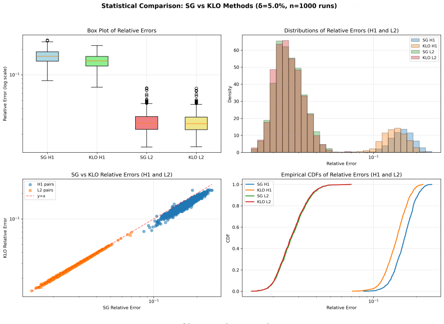
Statistical comparison of one thousand simulated reconstructions shows that the Sondhi-Gopinath method from 1971 produces lower error than the Korpela-Lassas-Oksanen method from 2016 when measurement noise is small, while the Korpela-Lassas-Oksanen method performs better once noise reaches higher levels; the Sondhi-Gopinath method is also easier to implement and runs faster.
What carries the argument
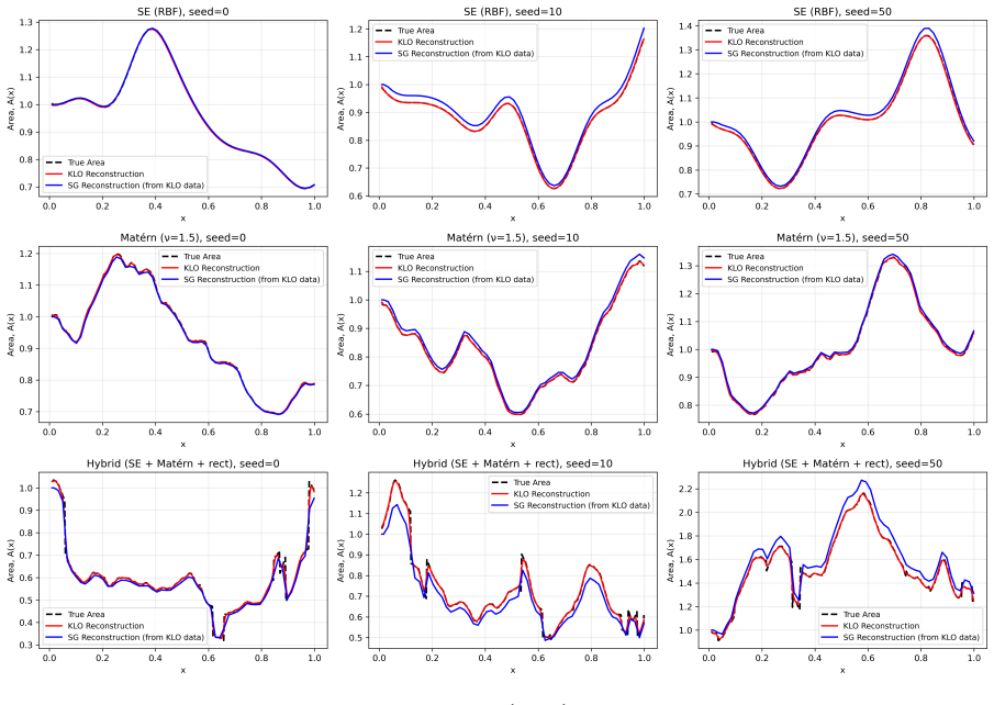
Two reconstruction algorithms (Sondhi-Gopinath and Korpela-Lassas-Oksanen) that each build solutions equal to the characteristic function of a spatial interval at a chosen time, using boundary observations of the wave equation.
If this is right
- The Sondhi-Gopinath method is the better practical choice when noise stays below a few percent of signal energy.
- The Korpela-Lassas-Oksanen method becomes preferable once noise exceeds roughly ten percent.
- Implementation effort and runtime favor the Sondhi-Gopinath method in settings where both accuracy and speed matter.
- The choice between the two methods should be made according to the expected noise level of the measurements.
Where Pith is reading between the lines
- The performance crossover may arise because each method processes a different order of time derivative of the boundary trace, so equalizing the input data order could change the observed ranking.
- Applying the same statistical protocol to other inverse problems governed by the wave equation, such as recovering speed or density, would test whether the noise-dependent advantage generalizes.
- Direct comparison on laboratory pipe data with independently verified area profiles would show whether the simulation ranking survives real sensor characteristics and model mismatch.
Load-bearing premise
The random area profiles and additive noise models used in the one thousand simulations accurately represent the real-world inverse boundary problem for pressurized fluid pipes, and the one time-derivative difference in the standard boundary data for the two methods does not introduce systematic bias.
What would settle it
Repeating the comparison on a fresh collection of one thousand profiles generated from a different random model, or on measured data from an actual pipe whose area is known independently, and finding that the relative performance ranking reverses at the reported noise thresholds.
Figures


read the original abstract
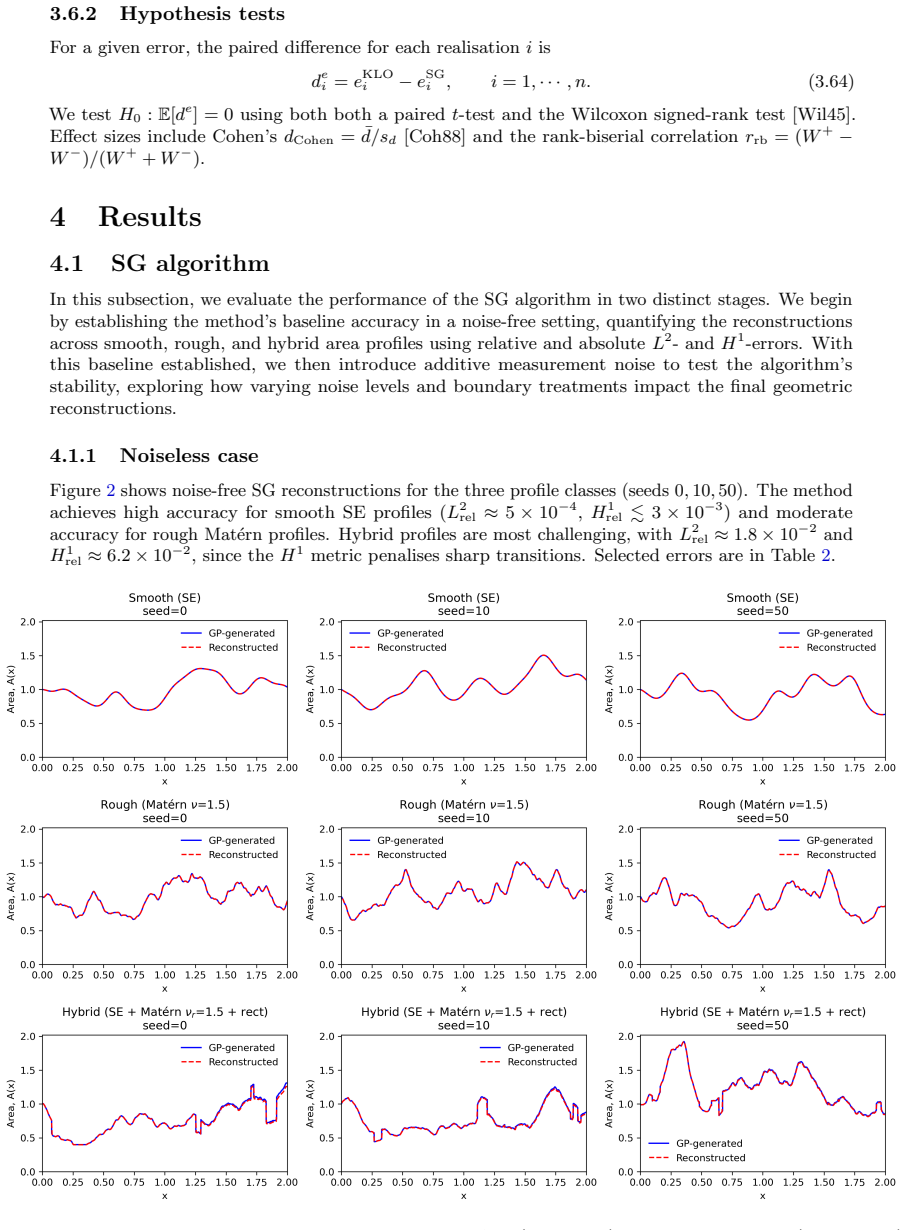
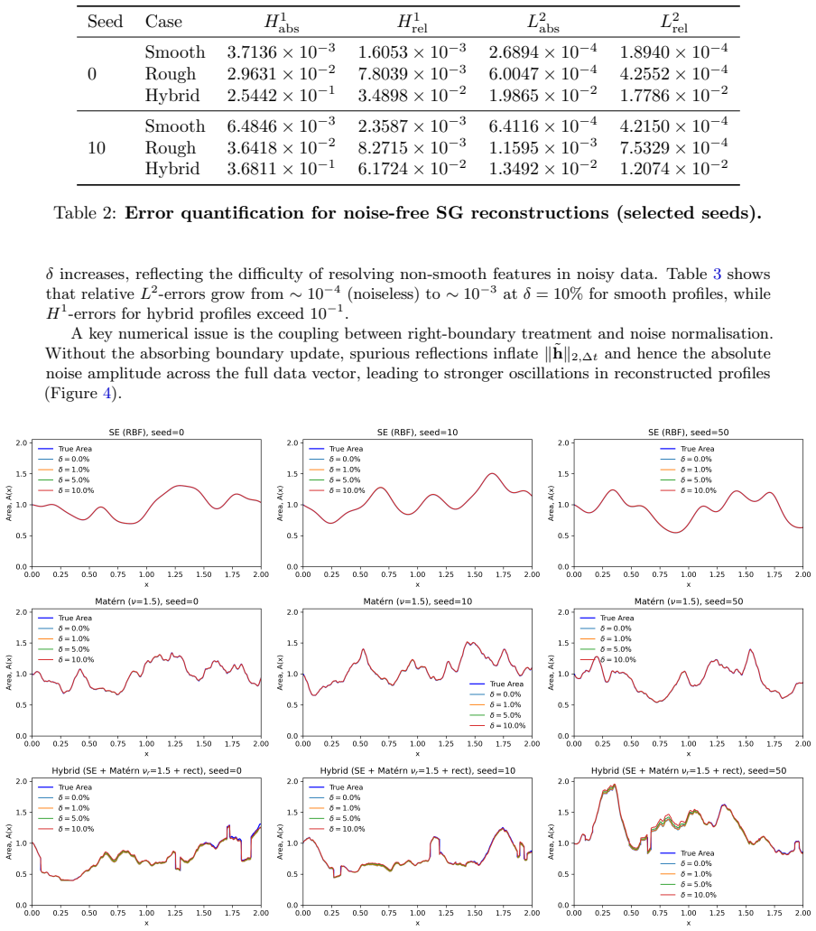
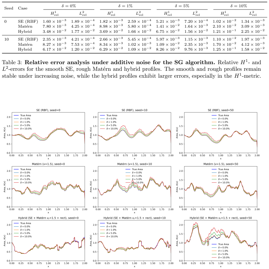
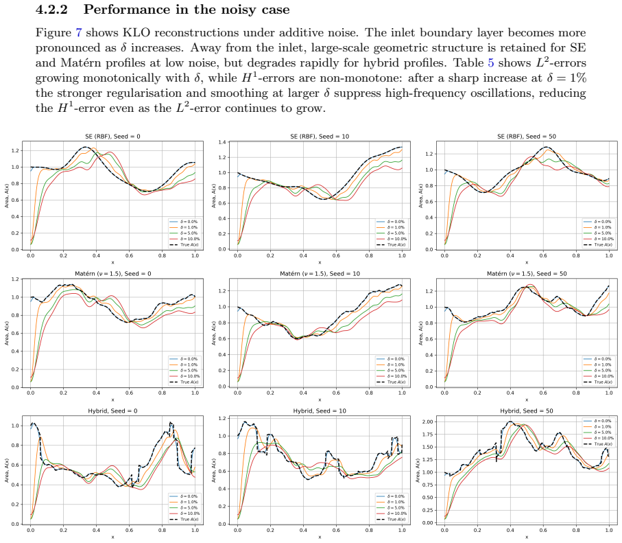
Several numerical reconstruction algorithms for the inverse boundary value problem of the 1-dimensional wave equation exist. In this paper we revisit two of them, the Sondhi-Gopinath (SG) method from 1971 and the Korpela-Lassas-Oksanen (KLO) method from 2016. The former is stable enough that it was used in practical applications. The latter has a regularisation scheme with a theoretical proof, and is an evolution of the boundary control method. Both are based on the idea of constructing solutions that are characteristic functions of a set at a given time. This similarity has been pointed out before, but no systematic comparison has been published. We compare the performance of the two algorithms with noisy simulated data. The application in our minds is reconstructing the internal cross-sectional area of a pressurised fluid pipe which corresponds to the first order $\partial_x$ term of the wave equation. Instead of just observing the performance on a few test cases, we generate $n=1000$ random area profiles of various smoothness levels and measurement noise up to $10\%$ of the signal energy and perform statistical tests. SG and KLO have a difference of one time-derivative in their standard boundary data, which complicates the analysis. Our results show that SG performs better in the low noise regime, and KLO with high noise. SG is easier to implement and runs faster.
Editorial analysis
A structured set of objections, weighed in public.
Referee Report
Summary. The manuscript presents a Monte-Carlo statistical comparison (n=1000) of the Sondhi-Gopinath (SG, 1971) and Korpela-Lassas-Oksanen (KLO, 2016) reconstruction algorithms for the inverse boundary problem of the 1D wave equation, motivated by pipe cross-section reconstruction. With simulated random area profiles and additive noise up to 10% of signal energy, the authors conclude that SG outperforms KLO in low-noise regimes while KLO is better at high noise; SG is also noted as simpler and faster to implement.
Significance. A rigorous head-to-head comparison of these methods could guide practical choices in applications like fluid pipe monitoring. The use of 1000 trials and statistical tests strengthens the evidence beyond anecdotal cases. The Monte-Carlo design with varied smoothness levels is a positive feature.
major comments (2)
- [Abstract and numerical experiments] Abstract and numerical experiments: noise is scaled to a fixed percentage of the energy of whichever boundary trace is supplied to each method. Because KLO receives the time derivative while SG receives the trace, differentiation amplifies high-frequency components, so the effective SNR seen by KLO is systematically lower than the nominal percentage. No section demonstrates re-scaling to equal L² energy or equal Sobolev regularity before the comparison, nor that the reported crossover (SG superior at low noise, KLO at high) survives such re-scaling.
- [Statistical analysis description] Statistical analysis description: the manuscript states that SG and KLO differ by one time derivative in their standard boundary data and that this 'complicates the analysis,' yet provides no explicit procedure for equalizing the noise models or for confirming that the regime-dependent ranking is not an artifact of the data convention.
minor comments (2)
- Clarify the precise definition of 'signal energy' used for noise scaling and the exact error metric (e.g., L² norm on the reconstructed area) reported in the statistical tests.
- The abstract could state the quantitative performance metrics and the precise statistical tests employed.
Simulated Author's Rebuttal
We thank the referee for the thoughtful and detailed report. The two major comments both concern the treatment of noise in the presence of the one-derivative difference between the standard data conventions of the two methods. We address each point below and outline the revisions we will make.
read point-by-point responses
-
Referee: [Abstract and numerical experiments] Abstract and numerical experiments: noise is scaled to a fixed percentage of the energy of whichever boundary trace is supplied to each method. Because KLO receives the time derivative while SG receives the trace, differentiation amplifies high-frequency components, so the effective SNR seen by KLO is systematically lower than the nominal percentage. No section demonstrates re-scaling to equal L² energy or equal Sobolev regularity before the comparison, nor that the reported crossover (SG superior at low noise, KLO at high) survives such re-scaling.
Authors: We agree that the effective noise level experienced by KLO is higher because its standard input is the time derivative of the trace supplied to SG. The manuscript uses the conventional data type for each algorithm precisely because that is how the methods are formulated and applied in the literature and in the motivating pipe-monitoring setting. Nevertheless, the referee correctly identifies that this choice leaves open the possibility that the observed crossover is partly an artifact of unequal effective SNR. To close this gap we will add a new subsection (provisionally 4.4) that repeats the Monte-Carlo study after re-scaling the additive noise so that both methods receive boundary data with identical L² energy (and, as a robustness check, identical H¹ energy). The statistical tests will be re-run on these equalized ensembles and the results reported alongside the original figures. revision: yes
-
Referee: [Statistical analysis description] Statistical analysis description: the manuscript states that SG and KLO differ by one time derivative in their standard boundary data and that this 'complicates the analysis,' yet provides no explicit procedure for equalizing the noise models or for confirming that the regime-dependent ranking is not an artifact of the data convention.
Authors: The manuscript notes the complication but does not supply the equalization procedure or the corresponding verification. In the revised version we will expand the statistical-analysis subsection to describe the re-scaling algorithm (additive white noise scaled to a target L² norm on the differentiated versus undifferentiated trace) and to present the outcome of the equalized comparison. If the crossover persists, that will be stated; if it does not, the revised text will qualify the original conclusion accordingly. revision: yes
Circularity Check
No circularity: empirical Monte-Carlo comparison is self-contained
full rationale
The paper's central claim (SG better at low noise, KLO at high noise) rests on 1000 independent random-profile simulations whose error metrics are computed directly from the generated data and reconstructions. No equation or result reduces by construction to a fitted input, self-citation chain, or ansatz. The acknowledged one-derivative difference in boundary data is handled by using each method's standard formulation; this is a methodological choice, not a definitional loop. External citations to the original SG (1971) and KLO (2016) papers supply the algorithms but do not bear the load of the new statistical ranking. The study is therefore self-contained against external benchmarks.
Axiom & Free-Parameter Ledger
Reference graph
Works this paper leans on
-
[1]
OPENGLOT – an Open Environment for the Evaluation of Glottal Inverse Filtering
[Alk+19] P Alku et al. “OPENGLOT – an Open Environment for the Evaluation of Glottal Inverse Filtering”. In:Speech Communication107.nil (2019), pp. 38–47.doi: 10.1016/j.specom.2019.01.005. [Alk11] P Alku. “Glottal Inverse Filtering Analysis of Human Voice Production — a Review of Estimation and Parameterization Methods of the Glottal Excitation and Their ...
-
[2]
Time and Frequency Domain Scattering for the One-Dimensional Wave Equation
Trudy Mat. Inst. Steklov. Engl. transl. 1971 Proc. Steklov Inst. Math. 115, 30–41. 1971, pp. 28–38. [Bro00] BL Browning. “Time and Frequency Domain Scattering for the One-Dimensional Wave Equation”. In:Inverse Problems16.5 (2000), pp. 1377–1403.doi: 10.1088/ 0266-5611/16/5/315. [Bro99] BL Browning. “Time and Frequency Domain Scattering for the One-Dimensi...
1971
-
[3]
On Characterization of Inverse Data in the Boundary Control Method
[BV16] MI Belishev and AF Vakulenko. “On Characterization of Inverse Data in the Boundary Control Method”. In:Rendiconti dell’Istituto di Matematica dell’Uni- versit` a di Trieste48 (2016), pp. 49–77.doi:10.13137/2464-8728/13151. [Coh88] J Cohen. “Statistical power analysis for the behavioral sciences New York”. In: NY: Academic54 (1988), pp. 77–155. [Dru...
-
[4]
Regularization Strategy for an Inverse Problem for a 1 + 1 Dimensional Wave Equation
[KLO16] J Korpela, M Lassas, and L Oksanen. “Regularization Strategy for an Inverse Problem for a 1 + 1 Dimensional Wave Equation”. In:Inverse Problems32.6 (Apr. 2016), p. 065001.doi:10.1088/0266-5611/32/6/065001. 27 [KS05] J Kaipio and E Somersalo.Statistical and Computational Inverse Problems. Vol
-
[5]
Scale-space for discrete signals
[Lin02] T Lindeberg. “Scale-space for discrete signals”. In:IEEE transactions on pattern analysis and machine intelligence12.3 (2002), pp. 234–254. [Lin24] T Lindeberg. “Discrete approximations of Gaussian smoothing and Gaussian derivatives”. In:Journal of Mathematical Imaging and Vision66.5 (2024), pp. 759–
2002
-
[6]
Webster's equation with curvature and dissipation
[LM12] T Lukkari and J Malinen. “Webster’s Equation With Curvature and Dissipation”. In:arXiv e-prints(2012). arXiv:1204.4075. [Oks11] L Oksanen. “Solving an Inverse Problem for the Wave Equation By Using a Minimization Algorithm and Time-Reversed Measurements”. In:Inverse Problems & Imaging5.3 (2011), pp. 731–744.doi:10.3934/ipi.2011.5.731. [Rak00] Rakes...
work page internal anchor Pith review Pith/arXiv arXiv doi:10.3934/ipi.2011.5.731 2012
-
[7]
Impedance Inversion From Transmission Data for the Wave Equation
[RS96] Rakesh and P Sacks. “Impedance Inversion From Transmission Data for the Wave Equation”. In:Wave Motion24.3 (1996), pp. 263–274.doi: 10.1016/s0165- 2125(96)00013-3. [Sch10] JB Schneider. “Understanding the finite-difference time-domain method”. In: School of electrical engineering and computer science Washington State University 28 (2010). [SG71] M ...
-
[8]
[SR83] MM Sondhi and J Resnick. “The Inverse Problem for the Vocal Tract: Numerical Methods, Acoustical Experiments, and Speech Synthesis”. In:The Journal of the Acoustical Society of America73.3 (1983), pp. 985–1002.doi: 10.1121/1.389024. [Ste99] ML Stein.Interpolation of spatial data: some theory for kriging. Springer Science & Business Media,
-
[9]
Unique Continuation for Solutions To Pde’s; Between H¨ ormander’s Theorem and Holmgren’s Theorem
[Tat95] D Tataru. “Unique Continuation for Solutions To Pde’s; Between H¨ ormander’s Theorem and Holmgren’s Theorem”. In:Communications in Partial Differential Equations20.5 (1995), pp. 855–884.doi:10.1080/03605309508821117. [Tat99] D Tataru. “Unique Continuation for Operatorswith Partially Analytic Coefficients”. In:Journal de Math´ ematiques Pures et Ap...
-
[10]
Individual comparisons by ranking methods
[Wil45] F Wilcoxon. “Individual comparisons by ranking methods”. In:Biometrics bulletin 1.6 (1945), pp. 80–83. [WR06] C Williams and C Rasmussen.Gaussian Processes for Machine Learning. Vol
1945
-
[11]
Internal Pipe Area Recon- struction As a Tool for Blockage Detection
[Zou+19] F Zouari, E Bl˚ asten, M Louati, and MS Ghidaoui. “Internal Pipe Area Recon- struction As a Tool for Blockage Detection”. In:Journal of Hydraulic Engineering 145.6 (June 2019), p. 04019019.doi:10.1061/(asce)hy.1943-7900.0001602. 28 [Zou+20] F Zouari, M Louati, S Meniconi, E Bl˚ asten, MS Ghidaoui, and B Brunone. “Experimental Verification of the ...
discussion (0)
Sign in with ORCID, Apple, or X to comment. Anyone can read and Pith papers without signing in.