Emergent Transfer of a Physics Foundation Model from Simulation to Laboratory Turbulence
Pith reviewed 2026-06-28 16:05 UTC · model grok-4.3
The pith
A foundation model finetuned on few DNS runs of Rayleigh-Taylor instability predicts the higher experimental mixing growth rates zero-shot on laboratory data.
A machine-rendered reading of the paper's core claim, the machinery that carries it, and where it could break.
Core claim
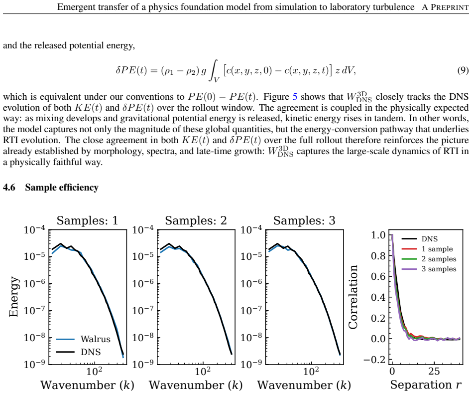
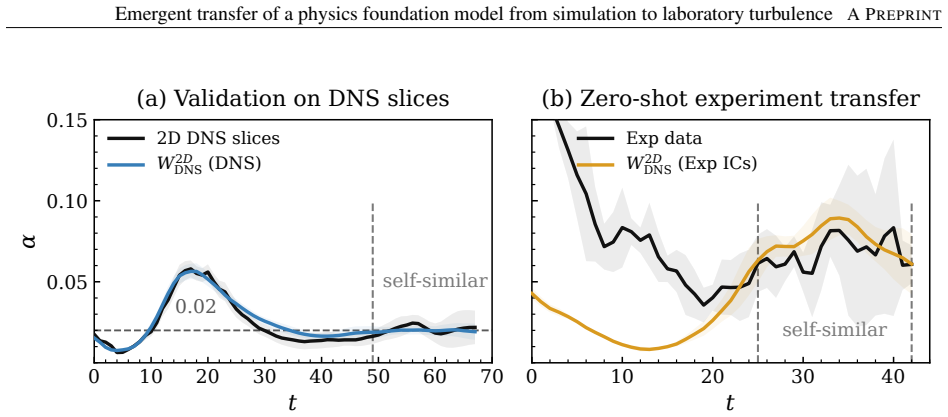
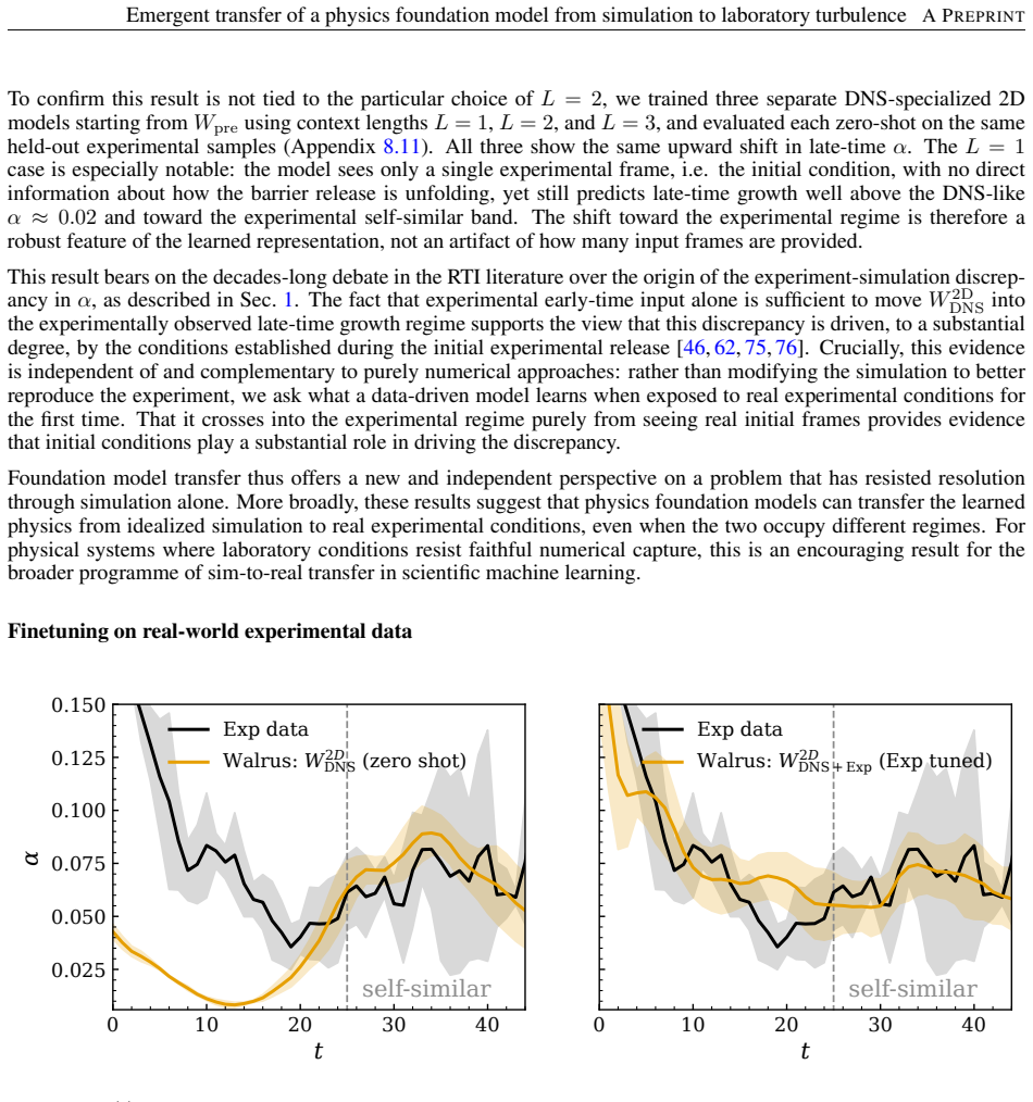
After finetuning on three or fewer DNS realizations, the Walrus foundation model for continuum dynamics recovers key Rayleigh-Taylor instability physics over long rollouts. When applied zero-shot to sliding-barrier laboratory data, the model leaves the DNS-like regime and enters the observed experimental growth band for alpha (~0.06-0.07), having seen no experimental samples. These results supply independent, data-driven evidence that initial conditions play a crucial role in the longstanding sim-experiment gap in alpha. The model additionally generalizes zero-shot to stable stratification, a buoyancy regime absent from training, and correctly slows mixing-layer growth.
What carries the argument
The Walrus foundation model for continuum dynamics, finetuned on a small number of DNS realizations and then applied zero-shot to experimental time series to predict mixing evolution.
If this is right
- The model can predict laboratory mixing behavior without ever seeing experimental training samples.
- Initial conditions are a primary driver of the discrepancy between simulation and experiment values of the mixing growth rate alpha.
- The same model can handle buoyancy regimes such as stable stratification that were never present in its training data.
- Foundation models trained exclusively on simulations can be deployed on sparse and noisy laboratory settings for fluid instabilities.
Where Pith is reading between the lines
- Similar few-shot finetuning on DNS could be used to probe initial-condition sensitivity in other fluid instabilities where simulation-experiment gaps persist.
- If the zero-shot transfer generalizes, it offers a route to test whether other experimental artifacts beyond initial conditions contribute to observed discrepancies.
- The efficiency with three or fewer DNS runs suggests that adaptation costs remain low even when extending the approach to additional laboratory configurations.
Load-bearing premise
The sliding-barrier laboratory data can be treated as directly comparable to idealized DNS without unaccounted differences in boundary conditions, measurement noise, or other experimental artifacts.
What would settle it
Measuring that the model's predicted alpha on the sliding-barrier laboratory data remains near the DNS value of ~0.02 instead of entering the 0.06-0.07 experimental band would falsify the transfer claim.
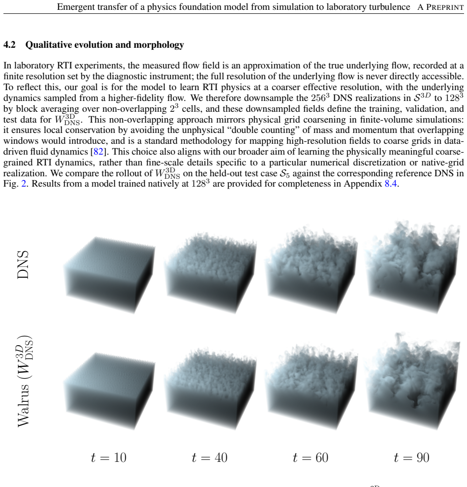
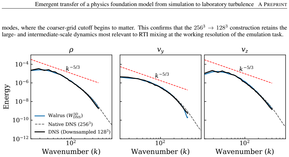
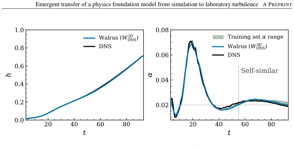
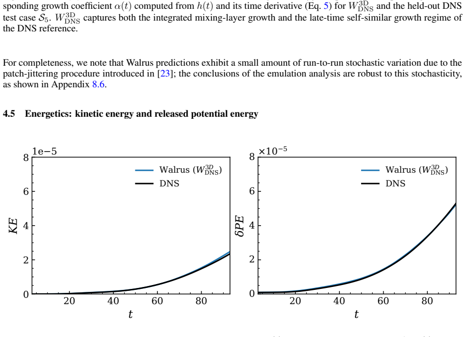
Figures


read the original abstract
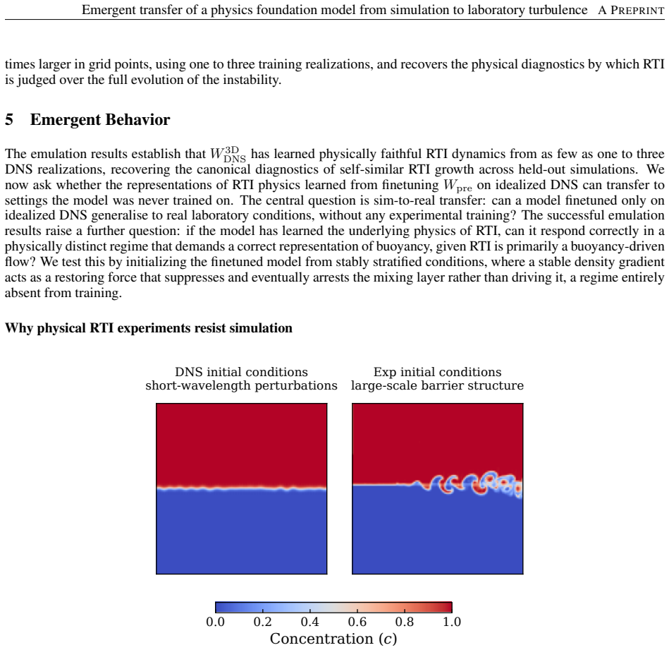
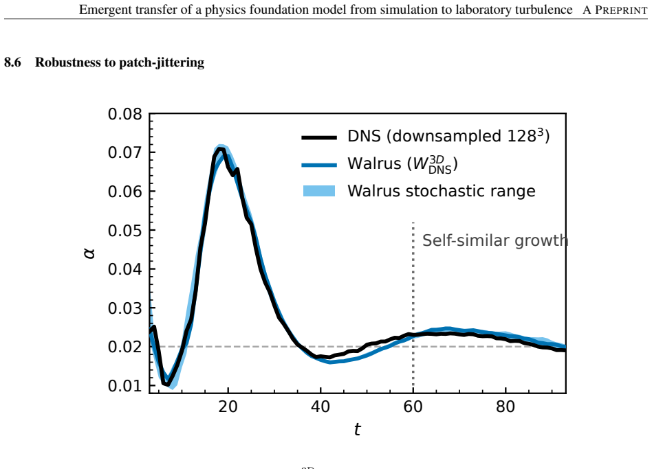
Whether physics foundation models can be usefully deployed on laboratory experiments remains an open question for scientific machine learning (ML). We test this question on the Rayleigh-Taylor instability (RTI), a ubiquitous and demanding fluid instability seen from tabletop flows to supernova explosions, in which small perturbations at a density interface grow into chaotic, multiscale mixing as a lighter fluid accelerates into a heavier one. Standard ML models struggle with RTI, and despite over a century of theoretical, numerical, and experimental work, it carries an unresolved discrepancy between simulation and experiment: the late-time mixing growth rate, $\alpha$, measured in most laboratory experiments ($\sim$ 0.06-0.07), is roughly three times the value from idealized direct numerical simulations (DNS, $\sim$ 0.02). The gap's origin remains debated. These properties make RTI a stringent test for a question that matters well beyond RTI: can foundation models trained only on simulations generalise to sparse, messy, and noisy laboratory settings? We finetune Walrus, a foundation model for continuum dynamics, on three or fewer DNS realizations and recover key RTI physics over long rollouts. Applied zero-shot to sliding-barrier laboratory data, the finetuned model leaves the DNS-like regime and enters the observed growth band, having never seen a single experimental sample. These results provide independent, data-driven evidence that initial conditions play a crucial role in the longstanding sim-experiment gap in $\alpha$. The model also generalises zero-shot to stable stratification, a buoyancy regime absent from training, correctly slowing mixing-layer growth. Together, our results show that foundation models can generalise well beyond their training data, predicting laboratory behavior and unseen physical regimes, opening new ways to probe longstanding simulation-experiment gaps.
Editorial analysis
A structured set of objections, weighed in public.
Referee Report
Summary. The paper claims that a foundation model (Walrus) finetuned on three or fewer DNS realizations of Rayleigh-Taylor instability recovers key physics over long rollouts; when applied zero-shot to sliding-barrier laboratory data, it produces a late-time mixing growth rate α in the experimental band (~0.06-0.07) rather than the DNS value (~0.02), supplying independent evidence that initial conditions explain the sim-experiment gap. The model also generalizes zero-shot to stable stratification, a regime absent from training.
Significance. If the central transfer result holds under rigorous controls, the work would demonstrate that physics foundation models trained solely on simulation can usefully predict laboratory behavior in a demanding, multiscale fluid instability, offering a new route to probe longstanding simulation-experiment discrepancies. The zero-shot generalization to an unseen buoyancy regime and the data-driven support for the role of initial conditions would be notable strengths for the field.
major comments (3)
- [§4] §4 (Laboratory data preparation): The claim that the observed α shift arises purely from differences in initial conditions requires that the laboratory perturbation spectrum, interface profile, and effective Atwood number are extracted and supplied without unaccounted mismatch; the manuscript provides no quantitative side-by-side comparison of these quantities between the sliding-barrier data and the DNS training set, which is load-bearing for the interpretation.
- [§5.1] §5.1 (Alpha extraction protocol): The reported entry into the experimental α band (0.06-0.07) is central to the headline result, yet the text does not demonstrate that the identical growth-rate measurement protocol (including any spatial averaging or time-window choices) is applied to both the model rollout and the laboratory reference data; any discrepancy here would undermine the direct comparison.
- [§5.3] §5.3 (Boundary-condition controls): The laboratory setup includes walls and end effects absent from the idealized DNS; without explicit tests showing that these do not alter the effective growth rate when the model is driven by the lab initial conditions, the attribution of the α change solely to initial conditions remains at risk.
minor comments (2)
- [Abstract] The abstract states 'three or fewer' DNS realizations but the main text should state the exact count used for the primary finetuning run to aid reproducibility.
- [Figures] Figure captions for the growth curves should explicitly label the DNS baseline, experimental reference band, and model prediction with consistent line styles and include uncertainty estimates where available.
Simulated Author's Rebuttal
We thank the referee for the careful and constructive report. The points raised highlight important aspects of rigor for the laboratory transfer claim. We respond to each major comment below and indicate the revisions planned.
read point-by-point responses
-
Referee: [§4] §4 (Laboratory data preparation): The claim that the observed α shift arises purely from differences in initial conditions requires that the laboratory perturbation spectrum, interface profile, and effective Atwood number are extracted and supplied without unaccounted mismatch; the manuscript provides no quantitative side-by-side comparison of these quantities between the sliding-barrier data and the DNS training set, which is load-bearing for the interpretation.
Authors: We agree that explicit quantitative comparisons are required to support the interpretation. In the revised manuscript we will add a new panel or table in §4 that directly compares (i) the initial perturbation power spectra obtained via consistent Fourier analysis, (ii) the initial interface thickness and shape profiles, and (iii) the effective Atwood numbers between the three DNS training realizations and the sliding-barrier laboratory data. Extraction methods will be documented to confirm no unaccounted mismatch. revision: yes
-
Referee: [§5.1] §5.1 (Alpha extraction protocol): The reported entry into the experimental α band (0.06-0.07) is central to the headline result, yet the text does not demonstrate that the identical growth-rate measurement protocol (including any spatial averaging or time-window choices) is applied to both the model rollout and the laboratory reference data; any discrepancy here would undermine the direct comparison.
Authors: We acknowledge that the protocol must be shown to be identical. The growth rate α is obtained from the same definition of mixing-layer width h(t) and the same linear regression in the self-similar regime, using identical time windows and spatial averaging. In the revision we will state the exact protocol (time interval, averaging domain, fitting procedure) explicitly in §5.1 and confirm its uniform application to both model rollouts and laboratory data, accompanied by supplementary h(t) curves for verification. revision: yes
-
Referee: [§5.3] §5.3 (Boundary-condition controls): The laboratory setup includes walls and end effects absent from the idealized DNS; without explicit tests showing that these do not alter the effective growth rate when the model is driven by the lab initial conditions, the attribution of the α change solely to initial conditions remains at risk.
Authors: This concern is valid. The laboratory measurements are taken from the central region, and the model is driven by lab initial conditions on a periodic domain approximating that region. We have not performed explicit wall-boundary tests. In the revision we will add a limitations paragraph in §5.3 discussing possible wall influence and, where computationally feasible, include a sensitivity test imposing approximate no-slip or damping boundaries to quantify any effect on α. We maintain that the primary change is driven by initial conditions, but will clarify the boundary assumptions. revision: partial
Circularity Check
No significant circularity; central result is empirical generalization to external lab data
full rationale
The paper's load-bearing claim is that a model finetuned only on DNS, when fed sliding-barrier laboratory inputs zero-shot, produces an alpha value that falls inside the independently measured experimental band (0.06-0.07). This alpha is extracted from the model's rollout on new data and compared to an external experimental reference; it is not fitted to the target alpha, not defined in terms of itself, and not justified by a self-citation chain. The derivation chain therefore remains self-contained against external benchmarks, with no reduction of the reported prediction to the model's own inputs by construction.
Axiom & Free-Parameter Ledger
free parameters (1)
- finetuning dataset size
axioms (1)
- domain assumption Walrus has learned sufficiently general representations of fluid dynamics from its pre-training corpus to support effective finetuning and zero-shot transfer.
Reference graph
Works this paper leans on
-
[1]
Hudson, Ehsan Adeli, Russ Altman, Simran Arora, Sydney von Arx, Michael S
Rishi Bommasani, Drew A. Hudson, Ehsan Adeli, Russ Altman, Simran Arora, Sydney von Arx, Michael S. Bernstein, Jeannette Bohg, Antoine Bosselut, Emma Brunskill, Erik Brynjolfsson, Shyamal Buch, Dallas Card, Rodrigo Castellon, Niladri Chatterji, Annie Chen, Kathleen Creel, Jared Quincy Davis, Dora Demszky, Chris Donahue, Moussa Doumbouya, Esin Durmus, Stef...
2021
-
[2]
Pdebench: An extensive benchmark for scientific machine learning.Advances in Neural Information Processing Systems, 35:1596–1611, 2022
Makoto Takamoto, Timothy Praditia, Raphael Leiteritz, Daniel MacKinlay, Francesco Alesiani, Dirk Pfl ¨uger, and Mathias Niepert. Pdebench: An extensive benchmark for scientific machine learning.Advances in Neural Information Processing Systems, 35:1596–1611, 2022
2022
-
[3]
Dalziel, Drummond Buschman Fielding, Daniel Fortunato, Jared A
Ruben Ohana, Michael McCabe, Lucas Thibaut Meyer, Rudy Morel, Fruzsina Julia Agocs, Miguel Beneitez, Marsha Berger, Blakesley Burkhart, Stuart B. Dalziel, Drummond Buschman Fielding, Daniel Fortunato, Jared A. Goldberg, Keiya Hirashima, Yan-Fei Jiang, Rich Kerswell, Suryanarayana Maddu, Jonah M. Miller, Payel Mukhopadhyay, Stefan S. Nixon, Jeff Shen, Roma...
2024
-
[4]
Realpdebench: A benchmark for complex physical systems with real-world data
Peiyan Hu, Haodong Feng, Hongyuan Liu, Tongtong Yan, Wenhao Deng, Tianrun Gao, Rong Zheng, Haoren Zheng, Chenglei Yu, Chuanrui Wang, Kaiwen Li, Zhi-Ming Ma, Dezhi Zhou, Xingcai Lu, Dixia Fan, and Tailin Wu. Realpdebench: A benchmark for complex physical systems with real-world data. InThe Fourteenth Inter- national Conference on Learning Representations, ...
2026
-
[5]
Towards multi-spatiotemporal-scale generalized PDE modeling
Jayesh K Gupta and Johannes Brandstetter. Towards multi-spatiotemporal-scale generalized PDE modeling. Transactions on Machine Learning Research, 2023
2023
-
[6]
Pinnacle: A comprehensive benchmark of physics-informed neural networks for solving pdes
Zhongkai Hao, Jiachen Yao, Chang Su, Hang Su, Ziao Wang, Fanzhi Lu, Zeyu Xia, Yichi Zhang, Songming Liu, Lu Lu, et al. Pinnacle: A comprehensive benchmark of physics-informed neural networks for solving pdes. arXiv preprint arXiv:2306.08827, 2023
-
[7]
AirfRANS: High fidelity com- putational fluid dynamics dataset for approximating reynolds-averaged navier–stokes solutions
Florent Bonnet, Jocelyn Ahmed Mazari, Paola Cinnella, and patrick gallinari. AirfRANS: High fidelity com- putational fluid dynamics dataset for approximating reynolds-averaged navier–stokes solutions. InThirty-sixth Conference on Neural Information Processing Systems Datasets and Benchmarks Track, 2022
2022
-
[8]
Artur Toshev, Gianluca Galletti, Fabian Fritz, Stefan Adami, and Nikolaus A. Adams. Lagrangebench: A la- grangian fluid mechanics benchmarking suite. InThirty-seventh Conference on Neural Information Processing Systems Datasets and Benchmarks Track, 2023
2023
-
[9]
Hans Hersbach, Bill Bell, Paul Berrisford, Shoji Hirahara, Andr ´as Hor ´anyi, Joaqu ´ın Mu˜noz-Sabater, Julien Nicolas, Carole Peubey, Raluca Radu, Dinand Schepers, Adrian Simmons, Cornel Soci, Saleh Abdalla, Xavier Abellan, Gianpaolo Balsamo, Peter Bechtold, Gionata Biavati, Jean Bidlot, Massimo Bonavita, Giovanna Chiara, Per Dahlgren, Dick Dee, Michail...
1999
-
[10]
David Neelin, David Randall, Sara Shamekh, Mark A Taylor, Nathan Urban, Janni Yuval, Guang Zhang, and Michael Pritchard
Sungduk Yu, Walter Hannah, Liran Peng, Jerry Lin, Mohamed Aziz Bhouri, Ritwik Gupta, Bj ¨orn L¨utjens, Jus- tus Christopher Will, Gunnar Behrens, Julius Busecke, Nora Loose, Charles I Stern, Tom Beucler, Bryce Harrop, Benjamin R Hillman, Andrea Jenney, Savannah Ferretti, Nana Liu, Anima Anandkumar, Noah D Brenowitz, 18 Emergent transfer of a physics found...
2023
-
[11]
EA- GLE: Large-scale learning of turbulent fluid dynamics with mesh transformers
Steeven JANNY , Aur´elien B ´en´eteau, Madiha Nadri, Julie Digne, Nicolas THOME, and Christian Wolf. EA- GLE: Large-scale learning of turbulent fluid dynamics with mesh transformers. InThe Eleventh International Conference on Learning Representations, 2023
2023
-
[12]
Bubbleformer: Forecasting boiling with transformers
Sheikh Md Shakeel Hassan, Xianwei Zou, Akash Dhruv, and Aparna Chandramowlishwaran. Bubbleformer: Forecasting boiling with transformers. InThe Thirty-ninth Annual Conference on Neural Information Processing Systems Datasets and Benchmarks Track, 2026
2026
-
[13]
LIPS - learning industrial physical sim- ulation benchmark suite
Milad Leyli-abadi, Antoine Marot, J ´erˆome Picault, David Danan, Mouadh Yagoubi, Benjamin Donnot, Seif- Eddine Attoui, Pavel Dimitrov, Asma Farjallah, and Clement Etienam. LIPS - learning industrial physical sim- ulation benchmark suite. InThirty-sixth Conference on Neural Information Processing Systems Datasets and Benchmarks Track, 2022
2022
-
[14]
Turbulence in focus: Benchmarking scaling behavior of 3d volumetric super-resolution with BLASTNet 2.0 data
Wai Tong Chung, Bassem Akoush, Pushan Sharma, Alex Tamkin, Ki Sung Jung, Jacqueline Chen, Jack Guo, Davy Brouzet, Mohsen Talei, Bruno Savard, Alexei Y Poludnenko, and Matthias Ihme. Turbulence in focus: Benchmarking scaling behavior of 3d volumetric super-resolution with BLASTNet 2.0 data. InThirty-seventh Conference on Neural Information Processing Syste...
2023
-
[15]
A public turbulence database cluster and applications to study lagrangian evolution of velocity increments in turbulence.Journal of Turbulence, 9:N31, January 2008
Yi Li, Eric Perlman, Minping Wan, Yunke Yang, Charles Meneveau, Randal Burns, Shiyi Chen, Alexander Szalay, and Gregory Eyink. A public turbulence database cluster and applications to study lagrangian evolution of velocity increments in turbulence.Journal of Turbulence, 9:N31, January 2008
2008
-
[16]
Flowbench: A large scale benchmark for flow simulation over complex geometries, 2024
Ronak Tali, Ali Rabeh, Cheng-Hau Yang, Mehdi Shadkhah, Samundra Karki, Abhisek Upadhyaya, Suriya Dhak- shinamoorthy, Marjan Saadati, Soumik Sarkar, Adarsh Krishnamurthy, Chinmay Hegde, Aditya Balu, and Baskar Ganapathysubramanian. Flowbench: A large scale benchmark for flow simulation over complex geometries, 2024
2024
-
[17]
Poseidon: Efficient foundation models for PDEs
Maximilian Herde, Bogdan Raonic, Tobias Rohner, Roger K ¨appeli, Roberto Molinaro, Emmanuel de Bezenac, and Siddhartha Mishra. Poseidon: Efficient foundation models for PDEs. InThe Thirty-eighth Annual Confer- ence on Neural Information Processing Systems, 2024
2024
-
[18]
Multiple physics pretraining for spatiotemporal surrogate models
Michael McCabe, Bruno R ´egaldo-Saint Blancard, Liam Holden Parker, Ruben Ohana, Miles Cranmer, Al- berto Bietti, Michael Eickenberg, Siavash Golkar, Geraud Krawezik, Francois Lanusse, Mariel Pettee, Tiberiu Tesileanu, Kyunghyun Cho, and Shirley Ho. Multiple physics pretraining for spatiotemporal surrogate models. InThe Thirty-eighth Annual Conference on ...
2024
-
[19]
Mahoney, and Amir Gholami
Shashank Subramanian, Peter Harrington, Kurt Keutzer, Wahid Bhimji, Dmitriy Morozov, Michael W. Mahoney, and Amir Gholami. Towards foundation models for scientific machine learning: Characterizing scaling and transfer behavior. InAdvances in Neural Information Processing Systems, 2023
2023
-
[20]
Morph: Pde foundation models with arbitrary data modality.arXiv preprint arXiv:2509.21670, 2025
Mahindra Singh Rautela, Alexander Most, Siddharth Mansingh, Bradley C Love, Ayan Biswas, Diane Oyen, and Earl Lawrence. Morph: Pde foundation models with arbitrary data modality.arXiv preprint arXiv:2509.21670, 2025
-
[21]
Physix: A foundation model for physics simulations,
Tung Nguyen, Arsh Koneru, Shufan Li, et al. Physix: A foundation model for physics simulations.arXiv preprint arXiv:2506.17774, 2025
-
[22]
DPOT: Auto-regressive denoising operator transformer for large-scale PDE pre-training
Zhongkai Hao, Chang Su, Songming Liu, Julius Berner, Chengyang Ying, Hang Su, Anima Anandkumar, Jian Song, and Jun Zhu. DPOT: Auto-regressive denoising operator transformer for large-scale PDE pre-training. In Forty-first International Conference on Machine Learning, 2024
2024
-
[23]
Michael McCabe, Payel Mukhopadhyay, Tanya Marwah, Bruno Regaldo-Saint Blancard, Francois Rozet, Cris- tiana Diaconu, Lucas Meyer, Kaze W. K. Wong, Hadi Sotoudeh, Alberto Bietti, Irina Espejo, Rio Fear, Siavash Golkar, Tom Hehir, Keiya Hirashima, Geraud Krawezik, Francois Lanusse, Rudy Morel, Ruben Ohana, Liam Parker, Mariel Pettee, Jeff Shen, Kyunghyun Ch...
2026
-
[24]
PROSE-FD: A multimodal PDE foundation model for learning multiple operators for forecasting fluid dynamics
Yuxuan Liu, Jingmin Sun, Xinjie He, Griffin Pinney, Zecheng Zhang, and Hayden Schaeffer. PROSE-FD: A multimodal PDE foundation model for learning multiple operators for forecasting fluid dynamics. InNeurips 2024 Workshop Foundation Models for Science: Progress, Opportunities, and Challenges, 2024. 19 Emergent transfer of a physics foundation model from si...
2024
-
[25]
PDE-transformer: Efficient and versatile trans- formers for physics simulations
Benjamin Holzschuh, Qiang Liu, Georg Kohl, and Nils Thuerey. PDE-transformer: Efficient and versatile trans- formers for physics simulations. InForty-second International Conference on Machine Learning, 2025
2025
-
[26]
VICON: Vision in-context operator networks for multi-physics fluid dynamics prediction.Transactions on Machine Learning Research, 2026
Yadi Cao, Yuxuan Liu, Liu Yang, Rose Yu, Hayden Schaeffer, and Stanley Osher. VICON: Vision in-context operator networks for multi-physics fluid dynamics prediction.Transactions on Machine Learning Research, 2026
2026
-
[27]
Yeh, Jean Kossaifi, Kamyar Azizzadenesheli, and Anima Anandkumar
Md Ashiqur Rahman, Robert Joseph George, Mogab Elleithy, Daniel Leibovici, Zongyi Li, Boris Bonev, Colin White, Julius Berner, Raymond A. Yeh, Jean Kossaifi, Kamyar Azizzadenesheli, and Anima Anandkumar. Pre- training codomain attention neural operators for solving multiphysics PDEs. InThe Thirty-eighth Annual Con- ference on Neural Information Processing...
2024
-
[28]
Towards a foundation model for partial differential equations: Multi-operator learning and extrapolation, 2025
Jingmin Sun, Yuxuan Liu, Zecheng Zhang, and Hayden Schaeffer. Towards a foundation model for partial differential equations: Multi-operator learning and extrapolation, 2025
2025
-
[29]
DISCO: learning to DISCover an evolution operator for multi- physics-agnostic prediction
Rudy Morel, Jiequn Han, and Edouard Oyallon. DISCO: learning to DISCover an evolution operator for multi- physics-agnostic prediction. InForty-second International Conference on Machine Learning, 2025
2025
-
[30]
Test-time generalization for physics through neural operator splitting.ArXiv, abs/2602.00884, 2026
Louis Serrano, Jiequn Han, Edouard Oyallon, Shirley Ho, and Rudy Morel. Test-time generalization for physics through neural operator splitting.ArXiv, abs/2602.00884, 2026
-
[31]
Tadpole: Autoencoders as foundation models for 3d pdes with online learning, 2026
Qiang Liu, Felix Koehler, Benjamin Holzschuh, and Nils Thuerey. Tadpole: Autoencoders as foundation models for 3d pdes with online learning, 2026
2026
-
[32]
Ai for scientific discovery is a social problem.Patterns, 7(3):101497, March 2026
Georgia Channing and Avijit Ghosh. Ai for scientific discovery is a social problem.Patterns, 7(3):101497, March 2026
2026
-
[33]
D. H. Sharp. An overview of Rayleigh–Taylor instability.Physica D: Nonlinear Phenomena, 12:3–18, 1984
1984
-
[34]
Cabot and Andrew W
William H. Cabot and Andrew W. Cook. Reynolds number effects on Rayleigh–Taylor instability with possible implications for type ia supernovae.Nature Physics, 2:562–568, 2006
2006
-
[35]
Instabilities and mixing in inertial confinement fusion.Annual Review of Fluid Mechanics, 57:197–225, 2025
Ye Zhou, James D Sadler, and Omar A Hurricane. Instabilities and mixing in inertial confinement fusion.Annual Review of Fluid Mechanics, 57:197–225, 2025
2025
-
[36]
K. I. Read. Experimental investigation of turbulent mixing by Rayleigh–Taylor instability.Physica D: Nonlinear Phenomena, 12(1-3):45–58, 1984
1984
-
[37]
Snider and Malcolm J
Dale M. Snider and Malcolm J. Andrews. Rayleigh–Taylor and shear driven mixing with an unstable thermal stratification.Physics of Fluids, 6(10):3324–3336, 1994
1994
-
[38]
Ramaprabhu and M
P. Ramaprabhu and M. J. Andrews. Experimental investigation of Rayleigh–Taylor mixing at small atwood numbers.Journal of Fluid Mechanics, 502:233–271, 2004
2004
-
[39]
D. H. Olson and J. W. Jacobs. Experimental study of Rayleigh–Taylor instability with a complex initial pertur- bation.Physics of Fluids, 21(3):034103–034103–13, March 2009
2009
-
[40]
D. L. Youngs. Modelling turbulent mixing by Rayleigh–Taylor instability.Physica D: Nonlinear Phenomena, 37:270–287, 1989
1989
-
[41]
Dimonte and M
G. Dimonte and M. Schneider. Turbulent Rayleigh–Taylor instability experiments with variable acceleration. Physical Review E, 54:3740–3743, 1996
1996
-
[42]
S. B. Dalziel, P. F. Linden, and D. L. Youngs. Self-similarity and internal structure of turbulence induced by Rayleigh–Taylor instability.Journal of Fluid Mechanics, 399:1–48, 1999
1999
-
[43]
Mueschke and Oleg Schilling
Nicholas J. Mueschke and Oleg Schilling. Investigation of Rayleigh–Taylor turbulence and mixing using ex- perimentally measured initial conditions. I. comparison to experimental data.Physics of Fluids, 21(1):014106, 2009
2009
-
[44]
Glimm, D
J. Glimm, D. H. Sharp, T. Kaman, and H. Lim. New directions for Rayleigh–Taylor mixing.Philosophical Transactions of the Royal Society A, 371:20120183, 2013
2013
-
[45]
M. J. Andrews and S. B. Dalziel. Small atwood number Rayleigh–Taylor experiments.Philosophical Transac- tions of the Royal Society A, 368:1663–1679, 2010
2010
-
[46]
David L. Youngs. Rayleigh–Taylor mixing: direct numerical simulation and implicit large eddy simulation. Physica Scripta, 92(7):074006, 2017
2017
-
[47]
Youngs, Andris Dimits, Stephan Weber, Martin Marinak, Stephan Wunsch, Christopher Garasi, Allen Robinson, Malcolm J
Guy Dimonte, David L. Youngs, Andris Dimits, Stephan Weber, Martin Marinak, Stephan Wunsch, Christopher Garasi, Allen Robinson, Malcolm J. Andrews, Praveen Ramaprabhu, Alan C. Calder, Bruce Fryxell, Joseph Biello, L. Jon Dursi, Peter MacNeice, Kevin Olson, Paul Ricker, Robert Rosner, Frank Timmes, Henry Tufo, Yuan-Nan Young, and Michael Zingale. A compara...
2004
-
[48]
D. L. Youngs. Numerical simulation of mixing by Rayleigh–Taylor and Richtmyer–Meshkov instabilities.Laser and Particle Beams, 12(4):725–750, 1994
1994
-
[49]
Molecular mixing in Rayleigh–Taylor instability.Journal of Fluid Mechanics, 265:97–124, 1994
PF Linden, JM Redondo, and DL Youngs. Molecular mixing in Rayleigh–Taylor instability.Journal of Fluid Mechanics, 265:97–124, 1994
1994
-
[50]
Cook, William Cabot, and Paul L
Andrew W. Cook, William Cabot, and Paul L. Miller. The mixing transition in Rayleigh–Taylor instability. Journal of Fluid Mechanics, 511:333–362, 2004
2004
-
[51]
Gregory C. Burton. Study of ultrahigh atwood-number Rayleigh–Taylor mixing dynamics using the nonlinear large-eddy simulation method.Physics of Fluids, 23(4):045106, 2011
2011
-
[52]
V . P. Statsenko, Yu. V . Yanilkin, and V . A. Zhmaylo. Direct numerical simulation of turbulent mixing.Philo- sophical Transactions of the Royal Society A, 371:20120216, 2013
2013
-
[53]
Petersen
Daniel Livescu, Tie Wei, and Mark R. Petersen. Direct numerical simulations of Rayleigh–Taylor instability. Journal of Physics: Conference Series, 318(8):082007, 2011
2011
-
[54]
Livescu, J
D. Livescu, J. R. Ristorcelli, M. R. Petersen, and R. A. Gore. New phenomena in variable-density Rayleigh– Taylor turbulence.Physica Scripta, T142:014015, 2010
2010
-
[55]
D. L. Youngs. Application of MILES to Rayleigh–Taylor and Richtmyer–Meshkov mixing. InAIAA Paper 2003-4102, 2003
2003
-
[56]
D. L. Youngs. The density ratio dependence of self-similar Rayleigh–Taylor mixing.Philosophical Transactions of the Royal Society A, 371:20120173, 2013
2013
-
[57]
Rayleigh–Taylor and Richtmyer–Meshkov instability induced flow, turbulence, and mixing
Ye Zhou. Rayleigh–Taylor and Richtmyer–Meshkov instability induced flow, turbulence, and mixing. ii.Physics Reports, 723–725:1–160, 2017
2017
-
[58]
Cambridge University Press, 2024
Ye Zhou.Hydrodynamic Instabilities and Turbulence: Rayleigh–Taylor, Richtmyer–Meshkov, and Kelvin– Helmholtz Mixing. Cambridge University Press, 2024
2024
-
[59]
Fourier neural operator for parametric partial differential equations
Zongyi Li, Nikola Borislavov Kovachki, Kamyar Azizzadenesheli, Burigede liu, Kaushik Bhattacharya, An- drew Stuart, and Anima Anandkumar. Fourier neural operator for parametric partial differential equations. In International Conference on Learning Representations, 2021
2021
-
[60]
Multi-grid ten- sorized fourier neural operator for high- resolution PDEs.Transactions on Machine Learning Research, 2024
Jean Kossaifi, Nikola Borislavov Kovachki, Kamyar Azizzadenesheli, and Anima Anandkumar. Multi-grid ten- sorized fourier neural operator for high- resolution PDEs.Transactions on Machine Learning Research, 2024
2024
-
[61]
U-Net: Convolutional Networks for Biomedical Image Segmentation
Olaf Ronneberger, Philipp Fischer, and Thomas Brox. U-net: Convolutional networks for biomedical image segmentation.CoRR, abs/1505.04597, 2015
work page internal anchor Pith review Pith/arXiv arXiv 2015
-
[62]
Rayleigh–Taylor and Richtmyer–Meshkov instability induced flow, turbulence, and mixing
Ye Zhou. Rayleigh–Taylor and Richtmyer–Meshkov instability induced flow, turbulence, and mixing. i.Physics Reports, 720–722:1–136, 2017
2017
-
[63]
Mohan, Nicholas Daniel, Michael Chertkov, and Daniel Livescu
Arvind T. Mohan, Nicholas Daniel, Michael Chertkov, and Daniel Livescu. Spatio-temporal deep learning mod- els of 3D turbulence with physics informed diagnostics.Journal of Turbulence, 21(9–10):484–524, 2020
2020
-
[64]
Long-term predictions of turbulence by implicit U-Net enhanced Fourier neural operator.Physics of Fluids, 35(7):075145, 2023
Zhijie Li, Wenhui Peng, Zelong Yuan, and Jianchun Wang. Long-term predictions of turbulence by implicit U-Net enhanced Fourier neural operator.Physics of Fluids, 35(7):075145, 2023
2023
-
[65]
Prediction of turbulent channel flow using Fourier neural operator-based machine-learning strategy.Physical Review Fluids, 9:084604, 2024
Yunpeng Wang, Zhijie Li, Zelong Yuan, Wenhui Peng, Tianyuan Liu, and Jianchun Wang. Prediction of turbulent channel flow using Fourier neural operator-based machine-learning strategy.Physical Review Fluids, 9:084604, 2024
2024
-
[66]
Adam Subel, Ashesh Chattopadhyay, Yifei Guan, and Pedram Hassanzadeh. Data-driven subgrid-scale modeling of forced Burgers turbulence using deep learning with generalization to higher Reynolds numbers via transfer learning.Physics of Fluids, 33(3):031702, 2021
2021
-
[67]
Yifei Guan, Ashesh Chattopadhyay, Adam Subel, and Pedram Hassanzadeh. Stable a posteriori LES of 2D turbulence using convolutional neural networks: Backscattering analysis and generalization to higher Re via transfer learning.Journal of Computational Physics, 458:111090, 2022
2022
-
[68]
Explaining the physics of transfer learning in data-driven turbulence modeling.PNAS Nexus, 2(3):pgad015, 2023
Adam Subel, Yifei Guan, Ashesh Chattopadhyay, and Pedram Hassanzadeh. Explaining the physics of transfer learning in data-driven turbulence modeling.PNAS Nexus, 2(3):pgad015, 2023
2023
-
[69]
P3d: Highly scalable 3d neural sur- rogates for physics simulations with global context
Benjamin Holzschuh, Georg Kohl, Florian Redinger, and Nils Thuerey. P3d: Highly scalable 3d neural sur- rogates for physics simulations with global context. InThe Fourteenth International Conference on Learning Representations, 2026
2026
-
[70]
Vivek Oommen, Siavash Khodakarami, Aniruddha Bora, Zhicheng Wang, and George Em Karniadakis. Learning turbulent flows with generative models: Super-resolution, forecasting, and sparse flow reconstruction.arXiv preprint arXiv:2509.08752, 2025. 21 Emergent transfer of a physics foundation model from simulation to laboratory turbulenceA PREPRINT
-
[71]
Fourier neural operator for large eddy simulation of compressible Rayleigh–Taylor turbulence.Physics of Fluids, 36(7):075165, 2024
Tengfei Luo, Zhijie Li, Zelong Yuan, Wenhui Peng, Tianyuan Liu, Liangzhu Wang, and Jianchun Wang. Fourier neural operator for large eddy simulation of compressible Rayleigh–Taylor turbulence.Physics of Fluids, 36(7):075165, 2024
2024
-
[72]
PhD thesis, University of Cambridge, 2018
Christopher Brown.Exploring the effects of an obstruction on the evolution of the Rayleigh–Taylor Instability. PhD thesis, University of Cambridge, 2018
2018
-
[73]
George, J
E. George, J. Glimm, X.-L. Li, A. Marchese, and Z.-L. Xu. A comparison of experimental, theoretical, and nu- merical simulation Rayleigh–Taylor mixing rates.Proceedings of the National Academy of Sciences, 99(5):2587– 2592, 2002
2002
-
[74]
Stuart B. Dalziel. Rayleigh–Taylor instability: experiments with image analysis.Dynamics of Atmospheres and Oceans, 20(1):127–153, 1993. American Geophysical Union Ocean Sciences Meeting
1993
-
[75]
Ramaprabhu, Guy Dimonte, and M
P. Ramaprabhu, Guy Dimonte, and M. J. Andrews. A numerical study of the influence of initial perturbations on the turbulent Rayleigh–Taylor instability.Journal of Fluid Mechanics, 536:285–319, 2005
2005
-
[76]
Ramaprabhu, D
Guy Dimonte, P. Ramaprabhu, D. L. Youngs, M. J. Andrews, and R. Rosner. Recent advances in the turbulent Rayleigh–Taylor instabilitya).Physics of Plasmas, 12(5):056301, May 2005
2005
-
[77]
Fermi and J
E. Fermi and J. von Neumann. Taylor instability of incompressible liquids. part 1. Taylor instability of an incompressible liquid. part 2. Taylor instability at the boundary of two incompressible liquids. Technical report, United States Atomic Energy Commission / Los Alamos Scientific Laboratory, 8 1953
1953
-
[78]
D. L. Youngs. Numerical simulation of turbulent mixing by Rayleigh–Taylor instability.Physica D: Nonlinear Phenomena, 12:32–44, 1984
1984
-
[79]
J. R. Ristorcelli and T. T. Clark. Rayleigh–Taylor turbulence: self-similar analysis and direct numerical simula- tions.Journal of Fluid Mechanics, 507:213–253, 2004
2004
-
[80]
Th `ese de doctorat, ´Ecole normale sup´erieure de Cachan (ENS Cachan), 2011
Romain Watteaux.D ´etection des grandes structures turbulentes dans les couches de m´elange de type Rayleigh– Taylor en vue de la validation de mod`eles statistiques turbulents bi-structure. Th `ese de doctorat, ´Ecole normale sup´erieure de Cachan (ENS Cachan), 2011. HAL thesis ID: tel-00669707
2011
discussion (0)
Sign in with ORCID, Apple, or X to comment. Anyone can read and Pith papers without signing in.