Multimodal Transformer Based Generic Mixture Density Network for Scattering Timescale Estimation of Fast Radio Bursts
Pith reviewed 2026-06-28 09:14 UTC · model grok-4.3
The pith
A multimodal transformer model estimates scattering timescales for fast radio bursts by predicting full probability distributions from spectra and profiles.
A machine-rendered reading of the paper's core claim, the machinery that carries it, and where it could break.
Core claim
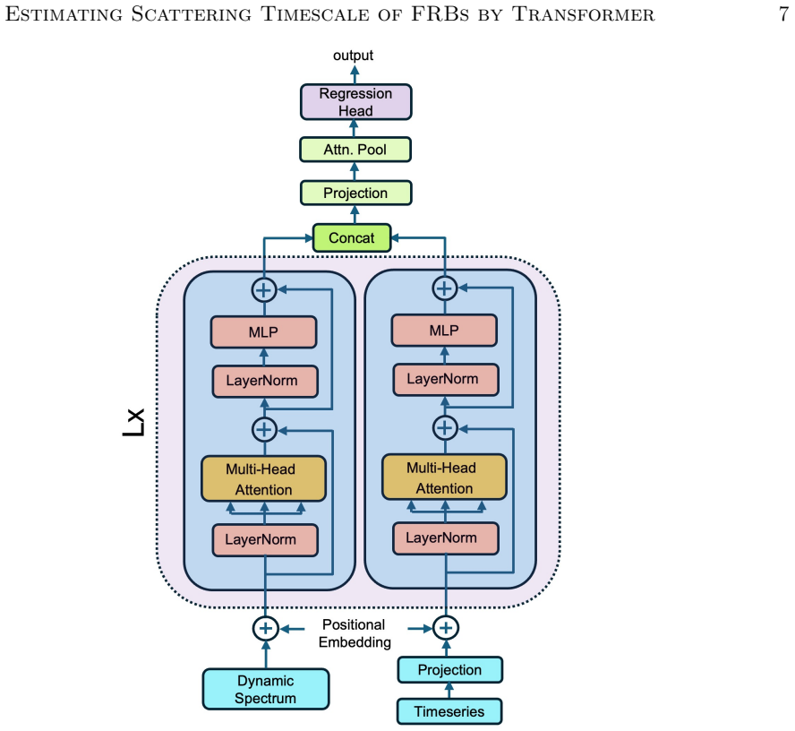
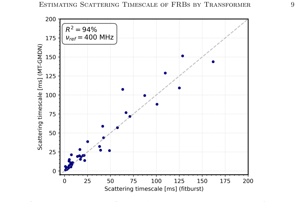
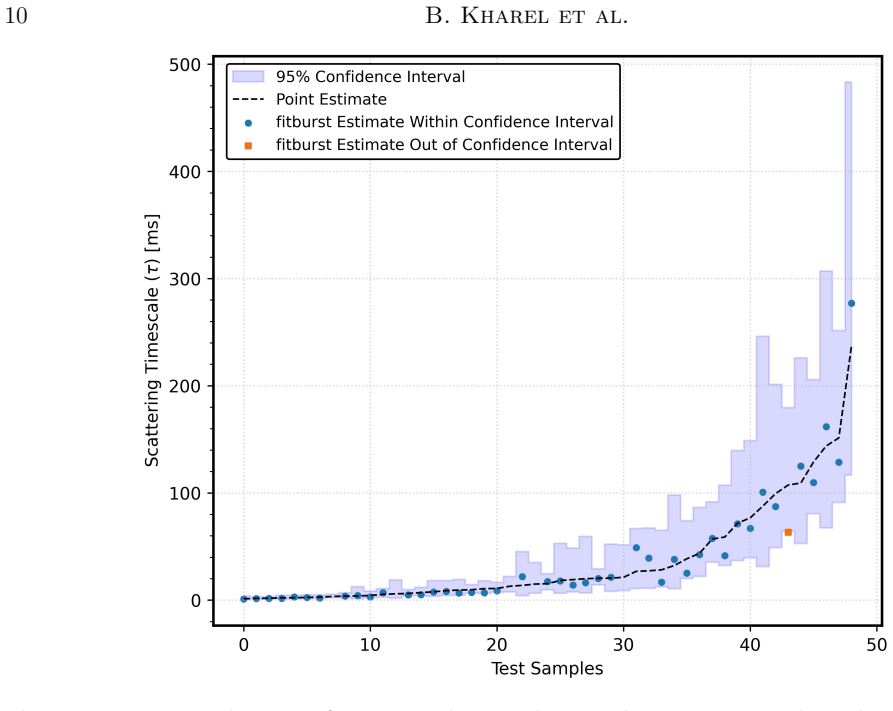
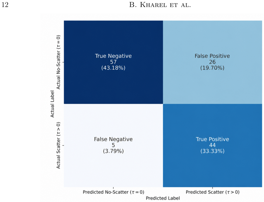
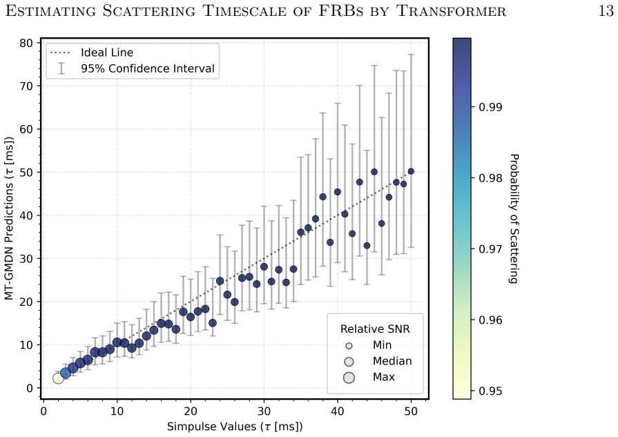
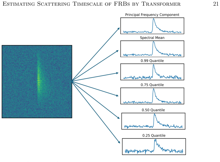
The MT-GMDN ingests the dynamic spectrum and timeseries profile through parallel transformer encoders, fuses their latent representations, and predicts the distribution of the scattering timescale using a generic mixture-density formulation. This captures both measurable scattering values and the zero-inflated population of bursts with unresolvable scattering. On held-out test data the expected values achieve a coefficient of determination of 94 percent with 90 percent recall, and the model incorporates heteroskedastic errors to allow confidence intervals.
What carries the argument
Multimodal Transformer Based Generic Mixture Density Network that runs parallel transformers on spectrum and profile inputs before fusing to a mixture density head for the scattering timescale.
If this is right
- The approach scales to large numbers of bursts without requiring manual supervision or careful initialization.
- It distinguishes bursts with measurable scattering from those without through the mixture components.
- Predictions come with uncertainty estimates derived from the output distributions and heteroskedastic modeling.
- Training on thousands of examples produces high accuracy on unseen data from the same survey.
Where Pith is reading between the lines
- Similar architectures could estimate other burst parameters such as dispersion measure or burst width.
- Deployment in real-time detection pipelines would enable immediate parameter reporting alongside discovery.
- Cross-validation against independent measurements from different instruments would test robustness beyond the training survey.
Load-bearing premise
The held-out events used for testing represent the statistical properties of future observations and the mixture-density formulation captures the zero-inflated population without overfitting to the training data.
What would settle it
Measuring the coefficient of determination and recall on an independent set of fast radio bursts observed with a different telescope and comparing against manual template fits; a substantial drop below 94 percent R-squared or 90 percent recall would indicate the model does not generalize.
Figures


read the original abstract
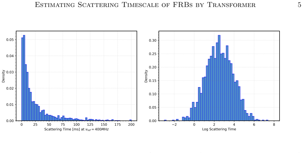
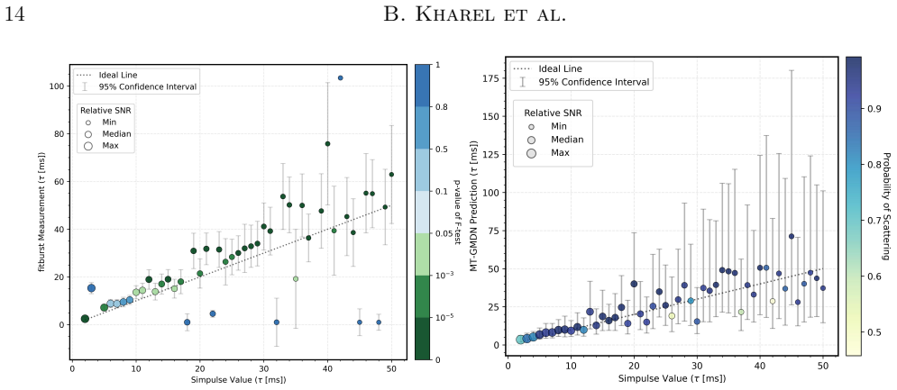
The discovery rate of fast radio bursts (FRBs) continues to increase with the advent of new radio facilities and yet extracting their astrophysical parameters such as scattering timescale ($\tau$) remains a significant bottleneck. Current $\tau$ measurement approaches like fitting analytic template models and scattering aware de-convolution are accurate but slow, sensitive to initialization, limited by low signal to noise and often require manual supervision. These limitations inspired us to explore fast, robust and scalable machine learning methods to estimate the astrophysical parameter value. We present a deep learning approach named Multimodal Transformer Based Generic Mixture Density Network (MT-GMDN) which ingests FRB dynamic spectrum and its corresponding timeseries profile through parallel transformer encoders, fuses their latent representations and predicts the distribution of $\tau$ with probabilistic output derived from generic mixture-density formulation. This formulation not only estimates the value of $\tau$ but also captures the (zero inflated) nature of FRB populations where a significant fraction of bursts exhibit unresolvable scattering. We trained MT-GMDN on $\sim3500$ FRBs from CHIME/FRB \cattwo while holding out some fraction of FRBs for validation during training and for testing after the training completes. The model achieves a coefficient of determination ($R^2$) value of $94\%$ on the expected value of $\tau$ for the events with measurable scattering with an excellent recall value of $90\%$ on the test data set. The model was also able to incorporate heteroskedastic errors enabling us the construction of a confidence interval for the predictions.
Editorial analysis
A structured set of objections, weighed in public.
Referee Report
Summary. The paper introduces MT-GMDN, a multimodal transformer architecture with parallel encoders for FRB dynamic spectra and time-series profiles, fused into a generic mixture-density network head that outputs a probabilistic distribution over scattering timescale τ. Trained on ~3500 CHIME/FRB events (with some fraction held out), the model reports R²=0.94 on expected τ for measurable events, 90% recall on the test set, and the ability to model zero-inflated populations plus heteroskedastic errors for confidence intervals.
Significance. If the generalization holds, the approach could accelerate τ estimation for growing FRB samples by replacing slow, initialization-sensitive template fitting with a fast, scalable probabilistic predictor. The mixture-density formulation for zero-inflated data and heteroskedastic uncertainty are positive features that could support downstream statistical analyses of FRB populations.
major comments (2)
- [Abstract] Abstract: The headline metrics (R²=0.94, recall=0.90) rest on a single held-out test fraction of the ~3500 events, but the abstract provides no description of the splitting procedure (temporal ordering, source-level blocking for repeaters, or explicit comparison of SNR/τ distributions between train and test). This directly affects whether the test set is representative of the zero-inflated population and future observations.
- [Abstract] Abstract: No details are supplied on network depth, loss function, hyperparameter search, or regularization; without these it is impossible to judge reproducibility or whether the reported performance is robust to low-SNR events, which the abstract itself identifies as a limitation of existing methods.
minor comments (1)
- [Abstract] Abstract: The token \cattwo is an unrendered LaTeX citation and should be replaced with a properly formatted reference.
Simulated Author's Rebuttal
We thank the referee for the constructive feedback. We address the two major comments on the abstract below and will revise the abstract in the next version to improve clarity on data handling and methodology while preserving its brevity.
read point-by-point responses
-
Referee: [Abstract] Abstract: The headline metrics (R²=0.94, recall=0.90) rest on a single held-out test fraction of the ~3500 events, but the abstract provides no description of the splitting procedure (temporal ordering, source-level blocking for repeaters, or explicit comparison of SNR/τ distributions between train and test). This directly affects whether the test set is representative of the zero-inflated population and future observations.
Authors: We agree the abstract should briefly indicate the splitting approach to support assessment of test-set representativeness. The manuscript details a random per-burst hold-out (with source-level blocking for repeaters and distribution matching on SNR and τ) in the data section; we will add a concise clause to the abstract summarizing this procedure and directing readers to the methods for full specifics. revision: yes
-
Referee: [Abstract] Abstract: No details are supplied on network depth, loss function, hyperparameter search, or regularization; without these it is impossible to judge reproducibility or whether the reported performance is robust to low-SNR events, which the abstract itself identifies as a limitation of existing methods.
Authors: We concur that the abstract would benefit from a short reference to core training choices to aid reproducibility judgments. These elements (transformer depth, mixture-density negative log-likelihood loss, hyperparameter tuning, and regularization) are fully specified in the methods; we will insert a brief parenthetical note in the abstract and retain the existing pointer to the detailed description. revision: yes
Circularity Check
No circularity: empirical ML performance on external telescope data
full rationale
The paper trains a multimodal transformer + mixture-density model on ~3500 CHIME/FRB events and reports R²=94% and 90% recall on a held-out test fraction. These metrics are direct empirical outcomes from external observational data; no derivation chain, equation, or first-principles result reduces by construction to fitted parameters, self-citations, or renamed inputs. No self-definitional steps, uniqueness theorems, or ansatzes smuggled via author citations appear in the reported claims. The result is therefore self-contained against external benchmarks.
Axiom & Free-Parameter Ledger
axioms (1)
- domain assumption The CHIME/FRB catalog events used for training and testing are representative of the broader FRB population and future observations.
Reference graph
Works this paper leans on
-
[1]
Lorimer, D. R., & Garver-Daniels, N. 2020, Monthly Notices of the Royal Astronomical Society, 497, 1661, doi: 10.1093/mnras/staa1856
-
[2]
Bhat, N. D. R., Cordes, J. M., & Chatterjee, S. 2003, ApJ, 584, 782, doi: 10.1086/345775
-
[3]
Bishop, C. M., & Bishop, H. 2024, Deep Learning: Foundations and Concepts (Springer), doi: 10.1007/978-3-031-45468-4 CHIME/FRB Collaboration, Amiri, M., Bandura, K., et al. 2018, ApJ, 863, 48, doi: 10.3847/1538-4357/aad188 CHIME/FRB Collaboration, Amiri, M., Bandura, K., et al. 2019, Nature, 566, 230, doi: 10.1038/s41586-018-0867-7 Chime/FRB Collaboration...
-
[4]
2018, The Astronomical Journal, 156, 256, doi: 10.3847/1538-3881/aae649
Connor, L., & van Leeuwen, J. 2018, The Astronomical Journal, 156, 256, doi: 10.3847/1538-3881/aae649
-
[5]
Cordes, J. M., & McLaughlin, M. A. 2003, ApJ, 596, 1142, doi: 10.1086/378231
-
[6]
Cordes, J. M., Ocker, S. K., & Chatterjee, S. 2022, Astrophys. J., 931, 88, doi: 10.3847/1538-4357/ac6873
-
[7]
Dosovitskiy, A., Beyer, L., Kolesnikov, A., et al. 2021, An Image is Worth 16x16 Words: Transformers for Image Recognition at Scale, https://arxiv.org/abs/2010.11929
Pith/arXiv arXiv 2021
-
[8]
Fonseca, E., Pleunis, Z., Andersen, B. C., et al. 2024, The Astrophysical Journal Supplement Series, 272, 7, doi: 10.3847/1538-4365/ad27d6
-
[9]
Harris, C. R., Millman, K. J., van der Walt, S. J., et al. 2020, Nature, 585, 357, doi: 10.1038/s41586-020-2649-2
-
[10]
The No-U-Turn Sampler: Adaptively Setting Path Lengths in Hamiltonian Monte Carlo
Hoffman, M. D., & Gelman, A. 2011, arXiv e-prints, arXiv:1111.4246, doi: 10.48550/arXiv.1111.4246
work page internal anchor Pith review Pith/arXiv arXiv doi:10.48550/arxiv.1111.4246 2011
-
[11]
2013, Applied Logistic Regression: Third Edition (wiley), doi: 10.1002/9781118548387
Hosmer, D., Lemeshow, S., & Sturdivant, R. 2013, Applied Logistic Regression: Third Edition (wiley), doi: 10.1002/9781118548387
-
[12]
Hunter, J. D. 2007, Computing in Science & Engineering, 9, 90, doi: 10.1109/MCSE.2007.55
-
[13]
2016, in MeerKAT Science: On the Pathway to the SKA, 1, doi: 10.22323/1.277.0001
Jonas, J., & MeerKAT Team. 2016, in MeerKAT Science: On the Pathway to the SKA, 1, doi: 10.22323/1.277.0001
-
[14]
Kharel, B., Fonseca, E., Brar, C., et al. 2025, Repeating vs. Non-Repeating FRBs: A Deep Learning Approach To Morphological Characterization, https://arxiv.org/abs/2509.06208
arXiv 2025
-
[15]
2015, Nature, 521, 436
LeCun, Y., Bengio, Y., & Hinton, G. 2015, Nature, 521, 436
2015
-
[16]
Narkevic, D. J., & Crawford, F. 2007,Science, 318, 777, doi: 10.1126/science.1147532
-
[17]
R., & Kramer, M
Lorimer, D. R., & Kramer, M. 2004, Handbook of Pulsar Astronomy, Vol. 4 (Cambridge, UK ; New York: Cambridge University Press)
2004
-
[18]
Macquart, J.-P., Bailes, M., Bhat, N. D. R., et al. 2010, PASA, 27, 272, doi: 10.1071/AS09082
-
[19]
McKinnon, M. M. 2014, Publications of the Astronomical Society of the Pacific, 126, 476, doi: 10.1086/676975
-
[20]
Ocker, S. K., Cordes, J. M., & Chatterjee, S. 2021, ApJ, 911, 102, doi: 10.3847/1538-4357/abeb6e
-
[21]
Ocker, S. K., Cordes, J. M., Chatterjee, S., et al. 2023, MNRAS, 519, 821, doi: 10.1093/mnras/stac3547 pandas development team, T. 2020, pandas-dev/pandas: Pandas, latest Zenodo, doi: 10.5281/zenodo.3509134
-
[22]
2026, ApJL, 1000, L53, doi: 10.3847/2041-8213/ae52f8
Pandhi, A., Nimmo, K., Andrew, S., et al. 2026, ApJL, 1000, L53, doi: 10.3847/2041-8213/ae52f8
-
[23]
2019, in Advances in Neural Information Processing Systems 32 (Curran Associates, Inc.), 8024–8035
Paszke, A., Gross, S., Massa, F., et al. 2019, in Advances in Neural Information Processing Systems 32 (Curran Associates, Inc.), 8024–8035
2019
-
[24]
2023, in American Astronomical Society Meeting
Sherman, M., & DSA-110 Collaboration. 2023, in American Astronomical Society Meeting
2023
-
[25]
Shin, K., Leung, C., Simha, S., et al. 2025, Astrophys. J., 993, 208 32B. Kharel et al. Shivraj Patil, S., Main, R. A., Fonseca, E., et al. 2025, arXiv e-prints, arXiv:2509.06721, doi: 10.48550/arXiv.2509.06721
-
[26]
2005, simpulse: C++/python library for simulating FRBs and pulsars,, https://github.com/kmsmith137/simpulse
Smith, K. 2005, simpulse: C++/python library for simulating FRBs and pulsars,, https://github.com/kmsmith137/simpulse
2005
-
[27]
1997, Introduction to Error Analysis, the Study of Uncertainties in Physical Measurements, 2nd Edition TorchVision maintainers and contributors
Taylor, J. 1997, Introduction to Error Analysis, the Study of Uncertainties in Physical Measurements, 2nd Edition TorchVision maintainers and contributors. 2016, TorchVision: PyTorch’s Computer Vision library,, https://github.com/pytorch/vision GitHub
1997
-
[28]
2023, Attention Is All You Need, https://arxiv.org/abs/1706.03762
Vaswani, A., Shazeer, N., Parmar, N., et al. 2023, Attention Is All You Need, https://arxiv.org/abs/1706.03762
Pith/arXiv arXiv 2023
-
[29]
Waskom, M. L. 2021, Journal of Open Source Software, 6, 3021, doi: 10.21105/joss.03021
-
[30]
Williamson, I. P. 1974, MNRAS, 166, 499, doi: 10.1093/mnras/166.3.499
-
[31]
2016, ApJ, 832, 199, doi: 10.3847/0004-637X/832/2/199
Xu, S., & Zhang, B. 2016, ApJ, 832, 199, doi: 10.3847/0004-637X/832/2/199
-
[32]
2025, A&A, 693, A85, doi: 10.1051/0004-6361/202450823
Yang, Tsung-Ching, Hashimoto, Tetsuya, Hsu, Tzu-Yin, et al. 2025, A&A, 693, A85, doi: 10.1051/0004-6361/202450823
discussion (0)
Sign in with ORCID, Apple, or X to comment. Anyone can read and Pith papers without signing in.