Spectral Scaling Laws of Muon
Pith reviewed 2026-06-28 11:16 UTC · model grok-4.3
The pith
Muon momentum matrices stabilize to layer-dependent power laws in model size after brief burn-in.
A machine-rendered reading of the paper's core claim, the machinery that carries it, and where it could break.
Core claim
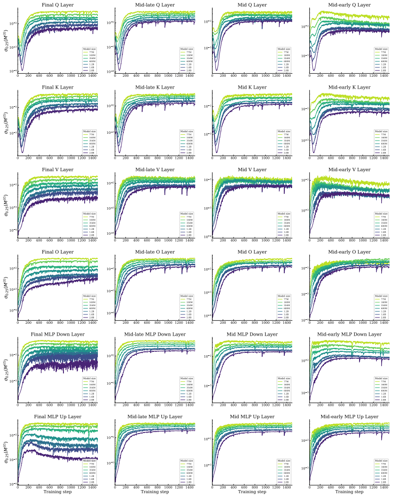
After a short burn-in, the quantiles of the singular value spectrum of the momentum buffer stabilize at values determined by layer type and model size; these stabilization values follow power laws in model size M with layer-dependent exponents, mild scaling around M^{-0.25} for layers up to mid-late depth and aggressive scaling up to M^{-0.96} for some late layers.
What carries the argument
Stabilization of singular-value quantiles of the momentum buffer to layer-dependent power laws in model size.
If this is right
- The standard five-step Newton-Schulz iteration will continue to orthonormalize layers up to mid-late depth at frontier model sizes.
- Late layers will require more Newton-Schulz iterations or retuned coefficients at large scales to avoid falling into the failure regime.
- The measured exponents allow a layer-aware choice of the minimal Newton-Schulz configuration that still orthonormalizes important directions without extra computation.
- The stabilization is a consistent property of the training dynamics across the tested range of model sizes.
Where Pith is reading between the lines
- If the exponents persist, training runs at 100B+ parameters will need depth-dependent Newton-Schulz iteration counts that increase toward the output layers.
- The clean power-law behavior suggests the training dynamics settle into a scale-invariant spectral regime after the burn-in phase.
- The same measurement protocol could be applied to other orthonormalized optimizers to test whether comparable layer-dependent scaling appears.
Load-bearing premise
The power-law exponents measured on models up to 2.8B parameters will continue to describe the singular-value stabilization behavior at frontier scales.
What would settle it
Train a model larger than 10B parameters, extract the singular-value quantiles of the momentum buffers in late layers, and check whether they lie on the extrapolated M^{-0.96} line from the 77M-2.8B data.
Figures


read the original abstract
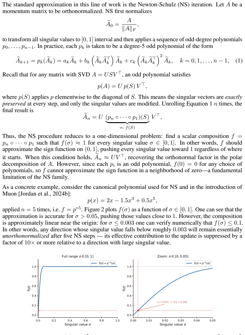
Orthonormalized update rules have rapidly become a leading choice of optimizer for training large language models, with recent open-source state-of-the-art models adopting Muon. To keep these updates tractable, Muon performs the orthonormalization with the Newton--Schulz (NS) iteration. Since NS is only approximate, directions with small singular values fail to be orthonormalized. In Muon, NS is applied to the momentum matrix at every step, yet little is known about how the singular value spectrum of these momentum matrices behaves during training, or how that behavior changes with model size. We present the first systematic study of this question. Tracking singular value quantiles of the momentum buffer across layers in models ranging from 77M to 2.8B parameters, we observe a consistent picture: after a short burn-in, the quantiles stabilize at a value determined by the layer type and model size. These stabilization values follow remarkably clean power laws in model size, with layer-dependent exponents. Layers up to mid-late depth scale very mildly with model size $M$ (around $M^{-0.25}$), so the standard 5-step NS configuration used at academic scale will continue to orthonormalize them at much larger scales. Some of the late layers, however, scale much more aggressively (up to $M^{-0.96}$) and will fall into the NS failure regime at frontier scale unless one uses more NS iterations or better-tuned coefficients. NS iterations are computationally expensive at scale; our laws give practitioners a principled, layer-aware recipe for choosing the minimum NS configuration that still orthonormalizes the directions that matter -- avoiding unnecessary computation without sacrificing update quality.
Editorial analysis
A structured set of objections, weighed in public.
Referee Report
Summary. The paper conducts the first systematic empirical study of singular-value quantiles in the momentum buffers of Muon-trained transformers. Tracking models from 77M to 2.8B parameters, it reports that after a short burn-in the quantiles stabilize to layer-dependent values that obey clean power-law scaling in model size M, with exponents ranging from approximately M^{-0.25} (early/mid layers) to M^{-0.96} (late layers). The authors conclude that standard 5-step Newton-Schulz (NS) will remain sufficient for most layers at frontier scale but that late layers will require additional iterations or retuned coefficients.
Significance. If the reported layer-dependent power laws continue to hold, the work supplies a practical, data-driven recipe for choosing minimal NS iteration counts per layer, which could reduce unnecessary orthonormalization cost at scale while preserving update quality. The systematic measurement across depth and size, together with the remarkably clean observed fits, constitutes a useful empirical contribution to the study of orthonormalized optimizers. The study remains purely observational; no theoretical derivation or closed-form prediction is offered.
major comments (2)
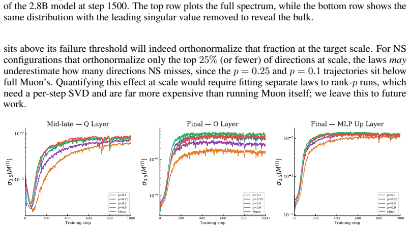
- [§4 and Figure 4] §4 (Scaling Laws) and Figure 4: The power-law exponents are obtained by fitting quantiles measured on models spanning only a factor of ~36 in size (77M–2.8B). The central claim that late layers will enter the NS failure regime at frontier scales rests on these exponents remaining invariant beyond the observed range; no runs at intermediate or larger scales, no ablation on data mix, learning-rate schedule, or NS coefficients, and no demonstration that the post-burn-in plateau is insensitive to initialization are provided.
- [§3.2] §3.2 (Quantile measurement protocol): The definition of the “stabilized” quantile (post-burn-in average) and the precise exclusion rules for early training steps are not stated with sufficient precision to allow independent reproduction or assessment of statistical significance of the reported exponents.
minor comments (2)
- [Table 1] Table 1: layer-depth binning boundaries are not explicitly listed; readers cannot map the reported exponents back to concrete layer indices without additional assumptions.
- [Figure 2] Figure 2 caption: the y-axis label “quantile” should specify whether it is the 0.01, 0.05, or median singular value to avoid ambiguity when comparing panels.
Simulated Author's Rebuttal
We thank the referee for the careful and constructive review. We respond point-by-point to the major comments below.
read point-by-point responses
-
Referee: [§4 and Figure 4] §4 (Scaling Laws) and Figure 4: The power-law exponents are obtained by fitting quantiles measured on models spanning only a factor of ~36 in size (77M–2.8B). The central claim that late layers will enter the NS failure regime at frontier scales rests on these exponents remaining invariant beyond the observed range; no runs at intermediate or larger scales, no ablation on data mix, learning-rate schedule, or NS coefficients, and no demonstration that the post-burn-in plateau is insensitive to initialization are provided.
Authors: We agree that the model-size range is limited and that the extrapolation to frontier scales assumes continued invariance of the observed exponents. The power-law fits are remarkably clean and consistent across layers within the studied range, which forms the core empirical contribution. We will add a limitations subsection explicitly discussing the restricted scale range, the assumptions required for extrapolation, and the desirability of future validation at larger scales. We cannot supply additional runs, ablations, or initialization-sensitivity tests at this time. revision: partial
-
Referee: [§3.2] §3.2 (Quantile measurement protocol): The definition of the “stabilized” quantile (post-burn-in average) and the precise exclusion rules for early training steps are not stated with sufficient precision to allow independent reproduction or assessment of statistical significance of the reported exponents.
Authors: We accept this criticism. The revised manuscript will state the protocol with full precision: the exact burn-in step threshold, the number of subsequent steps over which the quantile is averaged, the precise exclusion rule for early steps, and any associated statistical measures used to assess stability. revision: yes
- Additional experiments at larger model scales, ablations on data mix, learning-rate schedule, NS coefficients, and sensitivity of the post-burn-in plateau to initialization.
Circularity Check
No circularity; purely observational power-law fits on measured quantiles
full rationale
The paper measures singular-value quantiles of momentum buffers in models from 77M to 2.8B parameters, observes post-burn-in stabilization, and fits power laws in model size M with layer-dependent exponents. These are direct empirical fits to data; the reported stabilization values and exponents are not defined in terms of each other by any equation in the paper, nor do any 'predictions' for frontier scales reduce by construction to the fitted inputs. No self-citations, uniqueness theorems, or ansatzes are invoked as load-bearing steps. The derivation chain is self-contained observational analysis.
Axiom & Free-Parameter Ledger
free parameters (1)
- layer-dependent power-law exponents
axioms (1)
- domain assumption Singular-value quantiles of the momentum buffer reach a stable value after a short burn-in phase that is independent of further training steps.
Reference graph
Works this paper leans on
-
[1]
Disentangling adaptive gradient methods from learning rates.arXiv preprint arXiv:2002.11803,
Naman Agarwal, Rohan Anil, Elad Hazan, Tomer Koren, and Cyril Zhang. Disentangling adaptive gradient methods from learning rates.arXiv preprint arXiv:2002.11803,
-
[2]
Dion2: A simple method to shrink matrix in muon
Kwangjun Ahn, Noah Amsel, and John Langford. Dion2: A simple method to shrink matrix in muon. arXiv preprint arXiv:2512.16928, 2025a. Kwangjun Ahn, Byron Xu, Natalie Abreu, Ying Fan, Gagik Magakyan, Pratyusha Sharma, Zheng Zhan, and John Langford. Dion: Distributed orthonormalized updates.arXiv preprint arXiv:2504.05295, 2025b. Rohan Anil, Vineet Gupta, T...
-
[3]
URL https://leloykun.github. io/ponder/muon-opt-coeffs/. DeepSeek-AI. Deepseek-v3 technical report.arXiv preprint arXiv:2412.19437,
work page internal anchor Pith review Pith/arXiv arXiv
-
[4]
GLM-5: from Vibe Coding to Agentic Engineering
URL https://www. essential.ai/research/infra. GLM-5 Team. Glm-5: from vibe coding to agentic engineering.arXiv preprint arXiv:2602.15763,
work page internal anchor Pith review Pith/arXiv arXiv
-
[5]
Training Compute-Optimal Large Language Models
Jordan Hoffmann, Sebastian Borgeaud, Arthur Mensch, Elena Buchatskaya, Trevor Cai, Eliza Rutherford, Diego de Las Casas, Lisa Anne Hendricks, Johannes Welbl, Aidan Clark, et al. Training compute-optimal large language models.arXiv preprint arXiv:2203.15556,
work page internal anchor Pith review Pith/arXiv arXiv
-
[6]
Scaling Laws for Neural Language Models
Keller Jordan, Jeremy Bernstein, Brendan Rappazzo, @fernbear.bsky.social, Boza Vlado, You Jiacheng, Franz Cesista, Braden Koszarsky, and @Grad62304977. modded-nanogpt: Speedrunning the nanogpt baseline, 2024a. URLhttps://github.com/KellerJordan/modded-nanogpt. Keller Jordan, Yuchen Jin, Vlado Boza, Jiacheng You, Franz Cesista, Laker Newhouse, and Jeremy B...
work page internal anchor Pith review Pith/arXiv arXiv 2001
-
[7]
10 Kimi Team, Tongtong Bai, Yifan Bai, Yiping Bao, S. H. Cai, Yuan Cao, et al. Kimi k2.5: Visual agentic intelligence.arXiv preprint arXiv:2602.02276,
work page internal anchor Pith review Pith/arXiv arXiv
-
[8]
NorMuon: Making muon more efficient and scalable.arXiv preprint arXiv:2510.05491,
Zichong Li, Liming Liu, Chen Liang, Weizhu Chen, and Tuo Zhao. NorMuon: Making muon more efficient and scalable.arXiv preprint arXiv:2510.05491,
-
[9]
Muon is Scalable for LLM Training
Jingyuan Liu, Jianlin Su, Xingcheng Yao, Zhejun Jiang, Guokun Lai, Yulun Du, Yidao Qin, et al. Muon is scalable for llm training.arXiv preprint arXiv:2502.16982,
work page internal anchor Pith review Pith/arXiv arXiv
-
[10]
Llama Team. The llama 3 herd of models.arXiv preprint arXiv:2407.21783,
work page internal anchor Pith review Pith/arXiv arXiv
-
[11]
Hao-Jun Michael Shi, Tsung-Hsien Lee, Shintaro Iwasaki, Jose Gallego-Posada, Zhijing Li, Kaushik Rangadurai, Dheevatsa Mudigere, and Michael Rabbat. A distributed data-parallel PyTorch implementation of the distributed shampoo optimizer for training neural networks at-scale.arXiv preprint arXiv:2309.06497,
-
[12]
Team OLMo, Pete Walsh, Luca Soldaini, Dirk Groeneveld, Kyle Lo, et al. 2 olmo 2 furious.arXiv preprint arXiv:2501.00656,
work page internal anchor Pith review Pith/arXiv arXiv
-
[13]
Fantastic pretraining optimizers and where to find them.arXiv preprint arXiv:2509.02046,
Kaiyue Wen, David Hall, Tengyu Ma, and Percy Liang. Fantastic pretraining optimizers and where to find them.arXiv preprint arXiv:2509.02046,
-
[14]
Greg Yang, Edward J. Hu, Igor Babuschkin, Szymon Sidor, Xiaodong Liu, David Farhi, Nick Ryder, Jakub Pachocki, Weizhu Chen, and Jian Gao. Tensor programs V: Tuning large neural networks via zero-shot hyperparameter transfer.arXiv preprint arXiv:2203.03466,
-
[15]
A Appendix A.1 Details on pre-training We used the modded-nanogpt codebase [Jordan et al., 2024a] for all experiments. All matrix-valued parameters are trained with Muon, while non-matrix parameters (embeddings, LM head, and biases) are trained with AdamW with (β1, β2) = (0.9,0.95) and learning rate 0.002. For both optimizers we use a weight decay of 0.01...
2025
-
[16]
While this approximation is very good (see Figure 9), is uses 10 steps and hence is computationally more expensive
A.2.2 DeepSeek-V4 NS Coefficients [DeepSeek-AI, 2026] uses the following NS coefficients: a(x) = 2x−1.5x 3 + 0.5x5 c(x) = 3.4445x−4.7750x 3 + 2.0315x5 (3) The full NS map is then f=a ◦2 ◦c ◦8. While this approximation is very good (see Figure 9), is uses 10 steps and hence is computationally more expensive. 12 0.0 0.2 0.4 0.6 0.8 1.0 Singular value 0.0 0....
2026
discussion (0)
Sign in with ORCID, Apple, or X to comment. Anyone can read and Pith papers without signing in.