Quasi-birth-and-death processes evolving within trees: Applications to comparative phylogenetics
Pith reviewed 2026-06-28 03:08 UTC · model grok-4.3
The pith
An efficient recursive algorithm computes the likelihood of an observed phylogenetic tree under a quasi-birth-and-death model of discretized trait evolution.
A machine-rendered reading of the paper's core claim, the machinery that carries it, and where it could break.
Core claim
We develop an efficient recursive algorithm for computing the likelihood of an observed tree under this model where a QBD duplicates itself at fixed times within the tree, with the level obtained by discretizing a continuous trait and the phase modeling underlying environmental dynamics.
What carries the argument
Recursive algorithm that propagates likelihoods backward through the tree while accounting for QBD duplication at speciation nodes and transitions in levels and phases.
If this is right
- The algorithm yields the likelihood of any observed tree and its tip levels under the duplicating QBD model.
- Different choices of level discretization, phase rates, and duplication parameters produce a range of possible trait-evolution behaviors on the same tree.
- The framework supports analysis of partially observed states at the tips of empirical phylogenies.
- Application to the mammal data shows how likelihood changes with parameter values for range area and body size.
Where Pith is reading between the lines
- The same recursive structure could be used to compute likelihoods on non-phylogenetic trees provided duplication times are known.
- Sensitivity of the likelihood surface to the number of discretization levels could be checked by repeating the mammal analyses at finer and coarser partitions of the trait range.
- The phase variable offers a route to incorporate hidden environmental covariates without increasing the state space of the observed trait.
Load-bearing premise
Discretizing a continuous trait to obtain the QBD level variable preserves the essential dynamics of trait evolution.
What would settle it
Running the recursive likelihood algorithm on the same mammal phylogeny once with the discretized levels and once with a fully continuous-state model, then checking whether the two produce materially different maximum-likelihood parameter estimates or tree likelihood values.
Figures


read the original abstract
We consider a quasi-birth-and-process (QBD) that duplicates itself at some fixed times within a tree that contains information about duplication times and potentially partially observed states. We analyse a continuous trait by discretising it to obtain the QBD level variable. Then, the phase variable is used to model the dynamics of the underlying environment. Here, we extend the framework of Soewongsono et al. to enable a more general analysis. We develop an efficient recursive algorithm for computing the likelihood of an observed tree under this model and construct several numerical examples to illustrate its application potential. Through our synthetic data examples, we show a range of potential behaviours that could be modelled with this approach. Further, we apply the framework to two empirical examples from comparative phylogenetics (the evolution of range area and body size traits across a phylogeny of 49 mammals) to gain different insights into the evolution of these continuous traits. In this setting duplication of the QBD represents speciation and continuous trait evolution is modelled in a discretised state space. In our empirical examples, we explore the impact of different parameter choices on the corresponding likelihood of observing a given phylogenetic tree and the observed levels at its tips.
Editorial analysis
A structured set of objections, weighed in public.
Referee Report
Summary. The manuscript extends quasi-birth-and-death (QBD) processes to evolve on phylogenetic trees, with speciation corresponding to duplication events. A continuous trait is discretized to define the QBD level variable while the phase variable captures environmental dynamics; an efficient recursive algorithm is developed to compute the likelihood of an observed tree (with possible partial observations at tips), and the framework is illustrated on synthetic data plus two empirical mammalian phylogenies (range area and body size).
Significance. If the discretization step is shown to be a controlled approximation, the recursive likelihood algorithm would supply a new, computationally tractable way to embed state-dependent environmental effects into comparative phylogenetic models. The synthetic examples demonstrate a range of qualitative behaviors, and the empirical applications explore sensitivity to parameter choices, but the absence of any convergence analysis or error bounds for the discretization prevents assessment of whether the reported likelihoods and inferences remain reliable as approximations to continuous-trait dynamics.
major comments (2)
- [Abstract] Abstract (model-construction paragraph): the central modeling step obtains the QBD level by discretizing a continuous trait, yet no convergence argument, truncation-error bound, or preservation of key moments (e.g., expected change or variance) under the chosen rate matrices is supplied. Without such justification the recursive likelihood cannot be guaranteed to approximate the intended continuous-trait process on the tree.
- [Abstract] Abstract and empirical-examples paragraph: the two mammalian applications report likelihood sensitivity to parameter choices within the discretized model, but supply no comparison against standard continuous-trait models (Brownian motion, OU) or any diagnostic that the discretization preserves the qualitative features of the original trait data.
minor comments (1)
- [Abstract] Abstract: the phrase "quasi-birth-and-process (QBD)" is missing the word "death".
Simulated Author's Rebuttal
We thank the referee for the constructive comments on the discretization justification and empirical comparisons. We respond to each major comment below, indicating planned revisions where appropriate.
read point-by-point responses
-
Referee: [Abstract] Abstract (model-construction paragraph): the central modeling step obtains the QBD level by discretizing a continuous trait, yet no convergence argument, truncation-error bound, or preservation of key moments (e.g., expected change or variance) under the chosen rate matrices is supplied. Without such justification the recursive likelihood cannot be guaranteed to approximate the intended continuous-trait process on the tree.
Authors: We acknowledge that the manuscript lacks a formal convergence analysis or explicit error bounds. In revision we will add a dedicated subsection describing how the rate matrices are constructed to match the infinitesimal mean and variance of the underlying continuous process, together with numerical convergence checks (likelihood stabilization as the number of levels grows). A complete theoretical proof of convergence to the continuous limit lies beyond the present scope and will be noted as future work with appropriate references. revision: partial
-
Referee: [Abstract] Abstract and empirical-examples paragraph: the two mammalian applications report likelihood sensitivity to parameter choices within the discretized model, but supply no comparison against standard continuous-trait models (Brownian motion, OU) or any diagnostic that the discretization preserves the qualitative features of the original trait data.
Authors: We agree that benchmarking would strengthen the empirical section. The revised manuscript will include likelihood comparisons under Brownian motion and Ornstein-Uhlenbeck models fitted to the same mammalian phylogenies and traits, plus moment-matching diagnostics (mean, variance, and autocorrelation) between discretized QBD simulations and the original continuous trait data. revision: yes
Circularity Check
No significant circularity detected; derivation is self-contained algorithmic extension
full rationale
The paper's central contribution is an efficient recursive algorithm for the likelihood of an observed tree under a QBD process on a phylogeny, obtained by extending the framework of Soewongsono et al. The discretization of a continuous trait into QBD levels is presented explicitly as a modeling choice in the abstract and model construction, not as a derived result that loops back to its own inputs. No equations, fitted parameters, or self-citation chains are shown that would make any prediction or uniqueness claim equivalent to the inputs by construction. The self-citation is to prior work by different authors and serves as a starting point rather than a load-bearing justification that forces the new algorithm. The numerical examples and empirical applications explore behavior within the chosen model without reducing the likelihood computation to tautology. This is the common case of an independent algorithmic development on top of an external modeling framework.
Axiom & Free-Parameter Ledger
Reference graph
Works this paper leans on
-
[1]
Aksamit, M
A. Aksamit, M. M. O’Reilly, and Z. Palmowski. Sensitivities of some performance measures of quasi-birth-and-death processes.Stochastic Models, 2024
2024
-
[2]
Aksamit, M
A. Aksamit, M. M. O’Reilly, and Z. Palmowski. Random walk on a quadrant: mapping to a one-dimensional level-dependent quasi-birth-and-death process.Stochastic Models, 2025
2025
-
[3]
N. G. Bean, P. K. Pollett, and P. G. Taylor. Quasistationary distributions for level-dependent quasi- birth-and-death processes.Communications in Statistics. Part C: Stochastic Models, 16(5):511–541, 2000
2000
-
[4]
J. M. Beaulieu, D.-C. Jhwueng, C. Boettiger, and B. C. O’Meara. Modeling stabilizing selection: expanding the Ornstein–Uhlenbeck model of adaptive evolution.Evolution, 66(8):2369–2383, 2012
2012
-
[5]
Bright and P
L. Bright and P. G. Taylor. Calculating the equilibrium distribution in level dependent quasi-birth- and-death processes.Communications in Statistics. Stochastic Models, 11(3):497–525, 1995
1995
-
[6]
M. A. Butler and A. A. King. Phylogenetic comparative analysis: a modeling approach for adaptive evolution.The american naturalist, 164(6):683–695, 2004
2004
-
[7]
Den Iseger
P. Den Iseger. Numerical transform inversion using gaussian quadrature.Probability in the Engi- neering and Informational Sciences, 20(1):1–44, 2006
2006
-
[8]
Felsenstein
J. Felsenstein. Evolutionary trees from dna sequences: a maximum likelihood approach.Journal of molecular evolution, 17:368–376, 1981
1981
-
[9]
Felsenstein
J. Felsenstein. Phylogenies and the comparative method.The American Naturalist, 125(1):1–15, 1985
1985
-
[10]
Fletcher.Practical methods of optimization
R. Fletcher.Practical methods of optimization. John Wiley & Sons, 2000
2000
-
[11]
Garland, Theodore, P
J. Garland, Theodore, P. H. Harvey, and A. R. Ives. Procedures for the Analysis of Comparative Data Using Phylogenetically Independent Contrasts.Systematic Biology, 41(1):18–32, 03 1992
1992
-
[12]
T. F. Hansen. Stabilizing selection and the comparative analysis of adaptation.Evolution, 51(5):1341–1351, 1997
1997
-
[13]
He.Fundamentals of matrix-analytic methods, volume 365
Q.-M. He.Fundamentals of matrix-analytic methods, volume 365. Springer, 2014
2014
-
[14]
L. S. T. Ho and C. An´ e. Intrinsic inference difficulties for trait evolution with Ornstein-Uhlenbeck models.Methods in Ecology and Evolution, 5(11):1133–1146, 2014. 27
2014
-
[15]
Horv´ ath, I
G. Horv´ ath, I. Horv´ ath, S. A.-D. Almousa, and M. Telek. Numerical inverse Laplace transformation using concentrated matrix exponential distributions.Performance Evaluation, 137:102067, 2020
2020
-
[16]
Ingram and D
T. Ingram and D. L. Mahler. SURFACE: detecting convergent evolution from comparative data by fitting Ornstein-Uhlenbeck models with stepwise AIC.Methods in ecology and evolution, 4(5):416– 425, 2013
2013
-
[17]
Joyner and B
J. Joyner and B. Fralix. A new look at Markov processes of G/M/1-type.Stochastic Models, 32(2):253–274, 2016
2016
-
[18]
Latouche and V
G. Latouche and V. Ramaswami.Introduction to matrix analytic methods in stochastic modeling. SIAM, 1999
1999
-
[19]
J. A. Nelder and R. Mead. A simplex method for function minimization.The computer journal, 7(4):308–313, 1965
1965
-
[20]
M. F. Neuts.Matrix-geometric solutions in stochastic models: an algorithmic approach, volume 2 ofJohns Hopkins Series in the Mathematical Sciences. Johns Hopkins University Press, 1981
1981
-
[21]
H. K. Nigus.Stochastic Models for the Conservation of Endangered Species. PhD thesis, The University of Tasmania, Under preparation
-
[22]
Phung-Duc, H
T. Phung-Duc, H. Masuyama, S. Kasahara, and Y. Takahashi. A simple algorithm for the rate matrices of level-dependent QBD processes. In5th International Conference on Queueing Theory and Network Applications, QTNA 2010 - Proceedings, pages 46–52, 2010
2010
-
[23]
Ramaswami
V. Ramaswami. Matrix Analytic Methods: A Tutorial Overview with Some Extensions and New Results. InMatrix-Analytic Methods in Stochastic Models (Flint, MI), volume 183 ofLecture Notes in Pure and Appl. Math., pages 261–296. Dekker, New York, 1997
1997
-
[24]
L. J. Revell. phytools: an R package for phylogenetic comparative biology (and other things). Methods in Ecology and Evolution, (2):217–223, 2012
2012
-
[25]
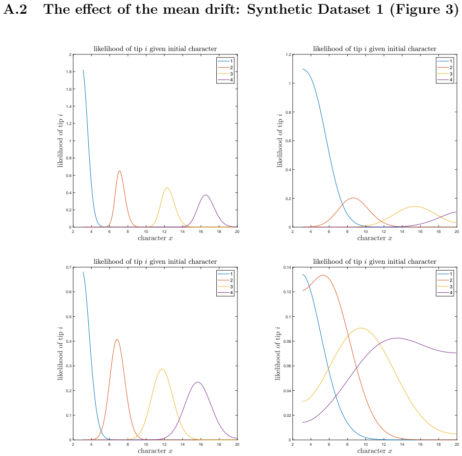
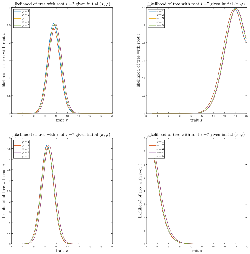
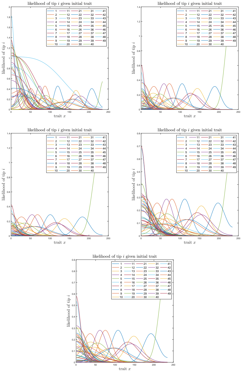
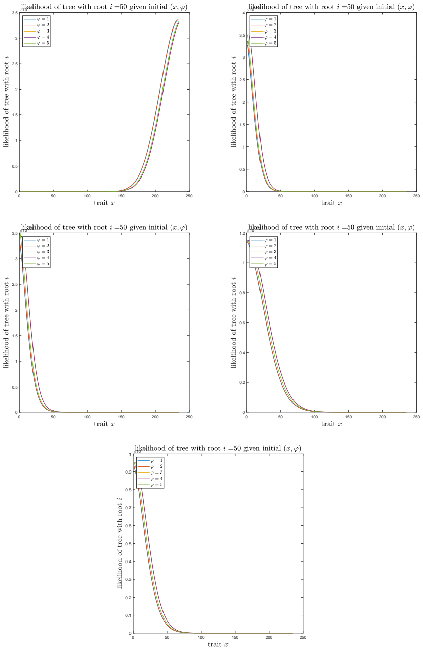
A. C. Soewongsono, J. Diao, T. Stark, A. E. Wilson, D. A. Liberles, B. R. Holland, and M. M. O’Reilly. Matrix-analytic methods for the evolution of species trees, gene trees, and their reconcil- iation.Methodology and Computing in Applied Probability, 27(1):1–47, 2025. 28 A The effect of the mean drift To illustrate the effect of the mean drift on the lik...
2025
discussion (0)
Sign in with ORCID, Apple, or X to comment. Anyone can read and Pith papers without signing in.