The SPHEREx View of Galaxy Clusters: A Simulation-based Validation of the Forced Photometry Pipeline for Extended Sources
Pith reviewed 2026-06-26 17:02 UTC · model grok-4.3
The pith
SPHEREx can measure cluster galaxy photometric redshifts to 0.003-0.01 precision and recover cluster redshifts to 0.002 scatter at low redshift.
A machine-rendered reading of the paper's core claim, the machinery that carries it, and where it could break.
Core claim
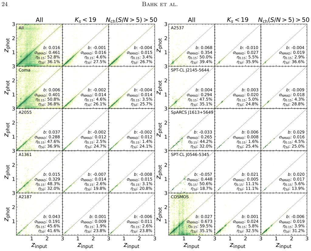
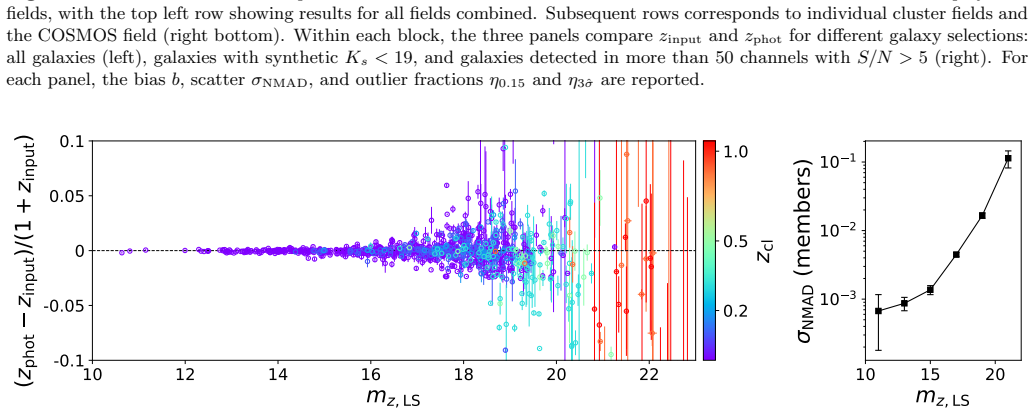
Through simulation of SPHEREx observations and application of forced photometry, the pipeline produces unbiased photometry for cluster members, with source blending as the main source of outliers. The survey reaches a depth of Ks ≈ 20 AB, sufficient to detect many members in low-redshift clusters but marginal at z ~ 1. With selection on brightness or signal-to-noise, cluster galaxy photometric redshifts achieve σ_NMAD ≈ 0.003-0.01, and stacking quality members recovers the cluster redshift with |Δz|/(1+z) < 0.002 bias and σ ≈ 0.002 scatter at z ≲ 0.5.
What carries the argument
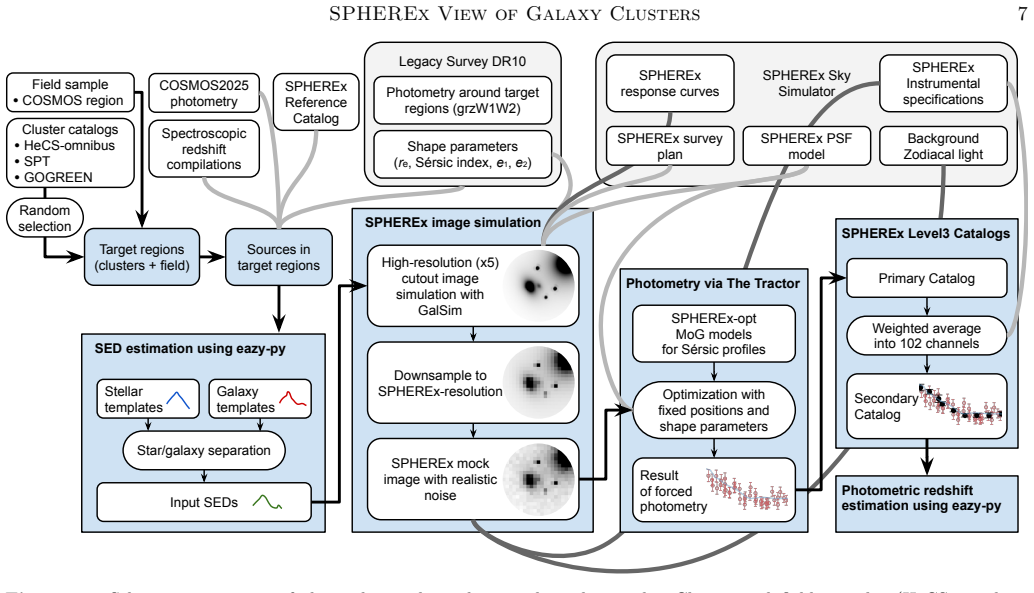
The end-to-end simulation pipeline that generates mock SPHEREx images with the SPHEREx Sky Simulator from DESI Legacy Survey and COSMOS ancillary data, followed by forced photometry using The Tractor.
If this is right
- Photometry remains generally unbiased despite blending challenges.
- Effective depth allows detection of members 7-9 magnitudes fainter than the BCG at low z.
- Appropriate sample selection based on brightness or S/N yields the quoted photo-z precision.
- Recovered cluster redshifts meet the precision needed for cluster cosmology at z ≲ 0.5.
Where Pith is reading between the lines
- Real SPHEREx data may require additional blending corrections if the simulation underestimates neighbor effects.
- The method could be applied to other large-scale structure probes beyond clusters.
- At higher redshifts, deeper ancillary data might be needed to maintain the same performance.
- This validation sets a benchmark for future space-based photometry missions targeting extended sources.
Load-bearing premise
The simulated observations accurately capture the real SPHEREx instrument's noise properties, point-spread function, and source blending statistics.
What would settle it
Comparison of actual SPHEREx flight photometry and derived redshifts against spectroscopic measurements for the same galaxy clusters.
Figures


read the original abstract
We present a simulation-driven assessment of the performance of the SPHEREx pipeline for galaxy cluster science, focusing on photometry, source blending, survey depth, and photometric redshift accuracy. To do that, we compile a sample of eight galaxy clusters spanning a wide redshift range ($z \approx 0.02$-$1.1$) and develop an end-to-end pipeline. We use the ancillary data from the DESI Legacy Survey and COSMOS survey, and generate realistic mock SPHEREx observations with the SPHEREx Sky Simulator. By performing forced photometry on these images with The Tractor, we quantify the characteristic biases and uncertainties relevant to cluster science. We find that the photometry is generally unbiased, but source blending is the primary driver of catastrophic outliers, particularly when the combined flux of neighbors is comparable to the flux of targets. Measuring the effective survey depth, we find that SPHEREx detects members down to $K_{s}\approx 20$ AB ($5\sigma$), 7-9 mag fainter than the brightest cluster galaxy (BCG) in nearby clusters but only 1-2 mag for clusters at $z \sim 1$, where the BCG itself has faded close to this depth. Despite these challenges, we demonstrate that SPHEREx can achieve a photometric redshift precision of $\sigma_{\mathrm{NMAD}}\approx 0.003$-$0.01$ for cluster galaxies with an appropriate sample selection based on brightness or signal-to-noise. Combining the redshifts of quality-selected members, we recover cluster redshifts with a bias of $|\Delta z|/(1+z) < 0.002$ and a scatter of $\sigma \approx 0.002$ at $z \lesssim 0.5$, meeting the precision required for cluster cosmology.
Editorial analysis
A structured set of objections, weighed in public.
Referee Report
Summary. The paper presents a simulation-driven assessment of the SPHEREx forced photometry pipeline for galaxy cluster science. Using mocks generated from DESI Legacy Survey and COSMOS data with the SPHEREx Sky Simulator for eight clusters at z ≈ 0.02-1.1, it performs forced photometry with The Tractor and evaluates biases, blending, depth, and photo-z accuracy. The key findings are that photometry is generally unbiased, blending drives catastrophic outliers when neighbor flux is comparable, SPHEREx reaches Ks≈20 AB depth, and with selection, achieves σ_NMAD≈0.003-0.01 for galaxy photo-z and cluster redshift recovery with |Δz|/(1+z) < 0.002 bias and σ ≈ 0.002 scatter at z ≲ 0.5.
Significance. If the simulation results hold, this provides a useful benchmark for SPHEREx cluster studies by identifying blending as the dominant error source and showing that the photometric precision needed for cluster cosmology can be reached at low redshift in the mocks. The end-to-end pipeline on realistic mocks is a strength.
major comments (1)
- [Abstract] Abstract: the headline performance metrics (σ_NMAD≈0.003-0.01 for galaxies; cluster redshift bias |Δz|/(1+z)<0.002 and scatter σ≈0.002 at z≲0.5) are obtained exclusively from forced photometry on SPHEREx Sky Simulator mocks; the manuscript provides no quantitative validation of the simulator's noise, PSF wings, or close-pair blending statistics against real data in dense fields, which is load-bearing for translating the results to flight data.
Simulated Author's Rebuttal
We thank the referee for their constructive review of our manuscript. We address the single major comment below and agree that additional caveats are warranted to properly contextualize the simulation results.
read point-by-point responses
-
Referee: [Abstract] Abstract: the headline performance metrics (σ_NMAD≈0.003-0.01 for galaxies; cluster redshift bias |Δz|/(1+z)<0.002 and scatter σ≈0.002 at z≲0.5) are obtained exclusively from forced photometry on SPHEREx Sky Simulator mocks; the manuscript provides no quantitative validation of the simulator's noise, PSF wings, or close-pair blending statistics against real data in dense fields, which is load-bearing for translating the results to flight data.
Authors: We agree that the manuscript does not include a quantitative validation of the SPHEREx Sky Simulator's noise properties, PSF wings, or close-pair blending statistics against real data in dense fields. The simulator is constructed from empirical inputs drawn from the DESI Legacy Survey and COSMOS catalogs, but this work does not perform a direct statistical comparison to observed dense-field data. Because the headline metrics are derived exclusively from these mocks, we will revise the abstract to include an explicit statement that the reported performance is obtained from simulated observations and will add a paragraph in the discussion section describing the simulator's assumptions and the need for future validation once flight data become available. These changes will better frame the applicability of the results to actual SPHEREx cluster studies. revision: yes
Circularity Check
No circularity: direct empirical comparison of pipeline outputs to known mock inputs
full rationale
The paper is a simulation-based validation study. It generates mock SPHEREx images from known ancillary catalogs (DESI Legacy Survey, COSMOS), runs forced photometry with The Tractor, and reports performance metrics by direct comparison to the input truth values. No derivations, parameter fits presented as predictions, or self-referential steps exist. The central claims (photo-z precision, cluster redshift recovery) are measured quantities from the mocks, not quantities that reduce to the inputs by construction. The simulator fidelity is an external modeling assumption, not a circularity issue.
Axiom & Free-Parameter Ledger
Reference graph
Works this paper leans on
-
[1]
Abbott, T. M. C., Aguena, M., Alarcon, A., et al. 2020, PhRvD, 102, 023509, doi: 10.1103/PhysRevD.102.023509 Abdurro’uf, Accetta, K., Aerts, C., et al. 2022, ApJS, 259, 35, doi: 10.3847/1538-4365/ac4414 42Bahk et al. LS DR10 Image High-Res Input SPHEREx-Res Input SPHEREx Mock Tractor Model Residual = 194.78 = 28.53 = 2.52 m 0.7 1 2 3 4 5 Wavelength [ m] 0...
-
[2]
2018, PhRvD, 98, 123529, doi: 10.1103/PhysRevD.98.123529
Aguena, M., & Lima, M. 2018, PhRvD, 98, 123529, doi: 10.1103/PhysRevD.98.123529
-
[3]
2026, The Open Journal of Astrophysics, 9, 55863, doi: 10.33232/001c.155863
Aguena, M., Aiola, S., Allam, S., et al. 2026, The Open Journal of Astrophysics, 9, 55863, doi: 10.33232/001c.155863
-
[4]
Akeson, R., Dubois-Felsmann, G. P., Crill, B. P., et al. 2025, arXiv e-prints, arXiv:2511.15823, doi: 10.48550/arXiv.2511.15823
-
[5]
Philosophical Transactions of the Royal Society of London Series A , keywords =
Allard, F., Homeier, D., & Freytag, B. 2012, Philosophical Transactions of the Royal Society of London Series A, 370, 2765, doi: 10.1098/rsta.2011.0269
-
[6]
Allen, S. W., Evrard, A. E., & Mantz, A. B. 2011, ARA&A, 49, 409, doi: 10.1146/annurev-astro-081710-102514
-
[7]
2025, https://arxiv.org/abs/2512.24537
Bae, J., Lee, B., Im, M., et al. 2025, https://arxiv.org/abs/2512.24537
arXiv 2025
-
[8]
Bahk, H., & Hwang, H. S. 2024, ApJS, 272, 7, doi: 10.3847/1538-4365/ad323f
-
[9]
Balogh, M. L., van der Burg, R. F. J., Muzzin, A., et al. 2021, MNRAS, 500, 358, doi: 10.1093/mnras/staa3008
-
[10]
B., Zengo, K., Ruel, J., et al
Bayliss, M. B., Zengo, K., Ruel, J., et al. 2017, ApJ, 837, 88, doi: 10.3847/1538-4357/aa607c
-
[11]
Beers, T. C., Flynn, K., & Gebhardt, K. 1990, AJ, 100, 32, doi: 10.1086/115487
-
[12]
Berlind, A. A., Frieman, J., Weinberg, D. H., et al. 2006, ApJS, 167, 1, doi: 10.1086/508170
-
[13]
2014, MNRAS, 443, 874, doi: 10.1093/mnras/stu1106
Bernardi, M., Meert, A., Vikram, V., et al. 2014, MNRAS, 443, 874, doi: 10.1093/mnras/stu1106
-
[14]
E., Stalder, B., de Haan, T., et al
Bleem, L. E., Stalder, B., de Haan, T., et al. 2015, ApJS, 216, 27, doi: 10.1088/0067-0049/216/2/27
-
[15]
Bleem, L. E., Klein, M., Abbot, T. M. C., et al. 2024, The Open Journal of Astrophysics, 7, 13, doi: 10.21105/astro.2311.07512
-
[16]
Bock, J. J., Aboobaker, A. M., Adamo, J., et al. 2025, arXiv e-prints, arXiv:2511.02985, doi: 10.48550/arXiv.2511.02985
-
[17]
Bocquet, S., Grandis, S., Bleem, L. E., et al. 2024, PhRvD, 110, 083510, doi: 10.1103/PhysRevD.110.083510
-
[18]
2021, eazy-py, 0.5.2 doi: 10.5281/zenodo.5012704
Brammer, G. 2021, eazy-py, 0.5.2 doi: 10.5281/zenodo.5012704
-
[19]
Brammer, G. B., van Dokkum, P. G., & Coppi, P. 2008, ApJ, 686, 1503, doi: 10.1086/591786
work page internal anchor Pith review doi:10.1086/591786 2008
-
[20]
Brown, M. J. I., Moustakas, J., Smith, J. D. T., et al. 2014, ApJS, 212, 18, doi: 10.1088/0067-0049/212/2/18
-
[21]
2025, arXiv e-prints, arXiv:2508.20332, doi: 10.48550/arXiv.2508.20332
Bryan, S., Bock, J., Burk, T., et al. 2025, arXiv e-prints, arXiv:2508.20332, doi: 10.48550/arXiv.2508.20332
-
[22]
2024, A&A, 685, A106, doi: 10.1051/0004-6361/202348264
Bulbul, E., Liu, A., Kluge, M., et al. 2024, A&A, 685, A106, doi: 10.1051/0004-6361/202348264
-
[23]
Casey, C. M., Kartaltepe, J. S., Drakos, N. E., et al. 2023, ApJ, 954, 31, doi: 10.3847/1538-4357/acc2bc
-
[24]
Chambers, K. C., Magnier, E. A., Metcalfe, N., et al. 2016, arXiv e-prints, arXiv:1612.05560, doi: 10.48550/arXiv.1612.05560
work page internal anchor Pith review Pith/arXiv arXiv doi:10.48550/arxiv.1612.05560 2016
-
[25]
2023, ApJ, 958, 118, doi: 10.3847/1538-4357/acf4a1
Chiang, Y.-K. 2023, ApJ, 958, 118, doi: 10.3847/1538-4357/acf4a1
-
[26]
2024, A&A, 687, A238, doi: 10.1051/0004-6361/202449447
Clerc, N., Comparat, J., Seppi, R., et al. 2024, A&A, 687, A238, doi: 10.1051/0004-6361/202449447
-
[27]
Condon, J. J. 1974, ApJ, 188, 279, doi: 10.1086/152714
-
[28]
Connolly, A. J., Csabai, I., Szalay, A. S., et al. 1995, AJ, 110, 2655, doi: 10.1086/117720
-
[29]
P., Werner, M., Akeson, R., et al
Crill, B. P., Werner, M., Akeson, R., et al. 2020, in Society of Photo-Optical Instrumentation Engineers (SPIE) Conference Series, Vol. 11443, Space Telescopes and Instrumentation 2020: Optical, Infrared, and Millimeter Wave, ed. M. Lystrup & M. D. Perrin, 114430I, doi: 10.1117/12.2567224
-
[30]
Crill, B. P., Bach, Y. P., Bryan, S. A., et al. 2025, arXiv e-prints, arXiv:2505.24856, doi: 10.48550/arXiv.2505.24856
-
[31]
The DESI Experiment Part I: Science,Targeting, and Survey Design
Dachan, K., Song, H., Kim, Y., et al. 2024, Journal of Korean Astronomical Society, 57, 45, doi: 10.5303/JKAS.2024.57.1.45 DESI Collaboration, Aghamousa, A., Aguilar, J., et al. 2016, arXiv e-prints, arXiv:1611.00036, doi: 10.48550/arXiv.1611.00036
work page internal anchor Pith review Pith/arXiv arXiv doi:10.5303/jkas.2024.57.1.45 2024
-
[32]
Cosmology with the SPHEREX All-Sky Spectral Survey
Dey, A., Schlegel, D. J., Lang, D., et al. 2019, AJ, 157, 168, doi: 10.3847/1538-3881/ab089d Dor´ e, O., Bock, J., Ashby, M., et al. 2014, arXiv e-prints, arXiv:1412.4872, doi: 10.48550/arXiv.1412.4872 Dor´ e, O., Werner, M. W., Ashby, M., et al. 2016, arXiv e-prints, arXiv:1606.07039, doi: 10.48550/arXiv.1606.07039 Dor´ e, O., Werner, M. W., Ashby, M. L....
work page internal anchor Pith review Pith/arXiv arXiv doi:10.3847/1538-3881/ab089d 2019
-
[33]
Dressler, A. 1980, ApJ, 236, 351, doi: 10.1086/157753
-
[34]
Duffy, A. R., Schaye, J., Kay, S. T., & Dalla Vecchia, C. 2008, MNRAS, 390, L64, doi: 10.1111/j.1745-3933.2008.00537.x
-
[35]
Ebeling, H., Edge, A. C., Bohringer, H., et al. 1998, MNRAS, 301, 881, doi: 10.1046/j.1365-8711.1998.01949.x
-
[36]
Eke, V. R., Baugh, C. M., Cole, S., et al. 2004, MNRAS, 348, 866, doi: 10.1111/j.1365-2966.2004.07408.x
-
[37]
Feder, R. M., Parker, L., & Seljak, U. 2026, arXiv e-prints, arXiv:2603.24668, doi: 10.48550/arXiv.2603.24668
-
[38]
Feder, R. M., Masters, D. C., Lee, B., et al. 2024, ApJ, 972, 68, doi: 10.3847/1538-4357/ad596d
-
[39]
2026, A&A, 709, A102, doi: 10.1051/0004-6361/202557708 44Bahk et al
Fumagalli, A., Costanzi, M., Castro, T., et al. 2026, A&A, 709, A102, doi: 10.1051/0004-6361/202557708 44Bahk et al. Gaia Collaboration, Prusti, T., de Bruijne, J. H. J., et al. 2016, A&A, 595, A1, doi: 10.1051/0004-6361/201629272
-
[40]
2009, A&A, 498, L33, doi: 10.1051/0004-6361/200911841
Gavazzi, R., Adami, C., Durret, F., et al. 2009, A&A, 498, L33, doi: 10.1051/0004-6361/200911841
-
[41]
2024, A&A, 689, A298, doi: 10.1051/0004-6361/202348852
Ghirardini, V., Bulbul, E., Artis, E., et al. 2024, A&A, 689, A298, doi: 10.1051/0004-6361/202348852
-
[42]
Gladders, M. D., & Yee, H. K. C. 2000, AJ, 120, 2148, doi: 10.1086/301557
-
[43]
, year = 1972, month = aug, volume =
Gunn, J. E., & Gott, III, J. R. 1972, ApJ, 176, 1, doi: 10.1086/151605
-
[44]
Haines, C. P., Pereira, M. J., Smith, G. P., et al. 2013, ApJ, 775, 126, doi: 10.1088/0004-637X/775/2/126
-
[45]
2021, ApJS, 253, 3, doi: 10.3847/1538-4365/abd023
Hilton, M., Sif´ on, C., Naess, S., et al. 2021, ApJS, 253, 3, doi: 10.3847/1538-4365/abd023
-
[46]
Ho, M., Ntampaka, M., Rau, M. M., et al. 2022, Nature Astronomy, 6, 936, doi: 10.1038/s41550-022-01711-1
-
[47]
Hogg, D. W., & Lang, D. 2013, PASP, 125, 719, doi: 10.1086/671228
-
[48]
Huai, Z., Bock, J. J., Cheng, Y.-T., et al. 2026, ApJ, 1000, 56, doi: 10.3847/1538-4357/ae472b
-
[49]
Huchra, J. P., & Geller, M. J. 1982, ApJ, 257, 423, doi: 10.1086/160000
-
[50]
Huterer, D., Kim, A., Krauss, L. M., & Broderick, T. 2004, ApJ, 615, 595, doi: 10.1086/424726
-
[51]
Huterer, D., & Shafer, D. L. 2018, Reports on Progress in Physics, 81, 016901, doi: 10.1088/1361-6633/aa997e
-
[52]
Hwang, H. S., Elbaz, D., Lee, J. C., et al. 2010, A&A, 522, A33, doi: 10.1051/0004-6361/201014807
-
[53]
Zahid, H. J. 2014, ApJ, 797, 106, doi: 10.1088/0004-637X/797/2/106
-
[54]
HyeongHan, K., Jee, M. J., Cha, S., & Cho, H. 2024, Nature Astronomy, 8, 377, doi: 10.1038/s41550-023-02164-w
-
[55]
Ilbert, O., Arnouts, S., McCracken, H. J., et al. 2006, A&A, 457, 841, doi: 10.1051/0004-6361:20065138
work page internal anchor Pith review doi:10.1051/0004-6361:20065138 2006
-
[56]
2009, ApJ, 690, 1236, doi: 10.1088/0004-637X/690/2/1236 Ivezi´ c,ˇZ., Kahn, S
Ilbert, O., Capak, P., Salvato, M., et al. 2009, ApJ, 690, 1236, doi: 10.1088/0004-637X/690/2/1236 Ivezi´ c,ˇZ., Kahn, S. M., Tyson, J. A., et al. 2019, ApJ, 873, 111, doi: 10.3847/1538-4357/ab042c
-
[57]
Kang, W., Hwang, H. S., Okabe, N., & Park, C. 2025, ApJS, 278, 51, doi: 10.3847/1538-4365/adcac8
-
[58]
2012, MNRAS, 427, 1344, doi: 10.1111/j.1365-2966.2012.22008.x
Kelvin, L. S., Driver, S. P., Robotham, A. S. G., et al. 2012, MNRAS, 421, 1007, doi: 10.1111/j.1365-2966.2012.20355.x
-
[59]
Khostovan, A. A., Kartaltepe, J. S., Salvato, M., et al. 2025, arXiv e-prints, arXiv:2503.00120, doi: 10.48550/arXiv.2503.00120
-
[60]
Kim, J. H., Im, M., Lee, H., et al. 2024, in Society of Photo-Optical Instrumentation Engineers (SPIE) Conference Series, Vol. 13094, Ground-based and Airborne Telescopes X, ed. H. K. Marshall, J. Spyromilio, & T. Usuda, 130940X, doi: 10.1117/12.3019546
-
[61]
Kim, T., Sohn, J., Hwang, H. S., et al. 2025, ApJS, 277, 41, doi: 10.3847/1538-4365/adb42a
-
[62]
Kitching, T. D., Miller, L., Heymans, C. E., van Waerbeke, L., & Heavens, A. F. 2008, MNRAS, 390, 149, doi: 10.1111/j.1365-2966.2008.13628.x
-
[63]
Klein, M., Mohr, J. J., Desai, S., et al. 2018, MNRAS, 474, 3324, doi: 10.1093/mnras/stx2929
-
[64]
2020, ApJS, 247, 43, doi: 10.3847/1538-4365/ab733b
Kluge, M., Neureiter, B., Riffeser, A., et al. 2020, ApJS, 247, 43, doi: 10.3847/1538-4365/ab733b
-
[65]
2024, A&A, 688, A210, doi: 10.1051/0004-6361/202349031
Kluge, M., Comparat, J., Liu, A., et al. 2024, A&A, 688, A210, doi: 10.1051/0004-6361/202349031
-
[66]
Koester, B. P., McKay, T. A., Annis, J., et al. 2007, ApJ, 660, 221, doi: 10.1086/512092
-
[67]
M., Bock, J
Korngut, P. M., Bock, J. J., Akeson, R., et al. 2018, in Society of Photo-Optical Instrumentation Engineers (SPIE) Conference Series, Vol. 10698, Space Telescopes and Instrumentation 2018: Optical, Infrared, and Millimeter Wave, ed. M. Lystrup, H. A. MacEwen, G. G
2018
-
[68]
Fazio, N. Batalha, N. Siegler, & E. C. Tong, 106981U, doi: 10.1117/12.2312860
-
[69]
Kornoelje, K., Bleem, L. E., Rykoff, E. S., et al. 2025, arXiv e-prints, arXiv:2503.17271, doi: 10.48550/arXiv.2503.17271
-
[70]
Kravtsov, A. V., & Borgani, S. 2012, ARA&A, 50, 353, doi: 10.1146/annurev-astro-081811-125502
-
[71]
M., Stebbins, A., Annis, J., et al
Kubo, J. M., Stebbins, A., Annis, J., et al. 2007, ApJ, 671, 1466, doi: 10.1086/523101 La Barbera, F., de Carvalho, R. R., de La Rosa, I. G., et al. 2010, MNRAS, 408, 1313, doi: 10.1111/j.1365-2966.2010.16850.x
-
[72]
2020, arXiv e-prints, arXiv:2012.15797, doi: 10.48550/arXiv.2012.15797
Lang, D. 2020, arXiv e-prints, arXiv:2012.15797, doi: 10.48550/arXiv.2012.15797
-
[73]
Lang, D., Hogg, D. W., & Schlegel, D. J. 2016b, AJ, 151, 36, doi: 10.3847/0004-6256/151/2/36
-
[74]
Lauer, T. R. 1999, PASP, 111, 1434, doi: 10.1086/316460
-
[75]
Euclid Definition Study Report
Laureijs, R., Amiaux, J., Arduini, S., et al. 2011, arXiv e-prints, arXiv:1110.3193, doi: 10.48550/arXiv.1110.3193
work page internal anchor Pith review Pith/arXiv arXiv doi:10.48550/arxiv.1110.3193 2011
-
[76]
Lee, J. H., Lee, M. G., Mun, J. Y., Cho, B. S., & Kang, J. 2022, ApJL, 931, L22, doi: 10.3847/2041-8213/ac6e39
-
[77]
Lee, J. H., Kim, M., Kim, T., et al. 2025, AJ, 169, 185, doi: 10.3847/1538-3881/adb285 SPHEREx View of Galaxy Clusters45
-
[78]
LSST Science Book, Version 2.0
Lima, M., & Hu, W. 2007, PhRvD, 76, 123013, doi: 10.1103/PhysRevD.76.123013 LSST Science Collaboration, Abell, P. A., Allison, J., et al. 2009, arXiv e-prints, arXiv:0912.0201, doi: 10.48550/arXiv.0912.0201
work page internal anchor Pith review Pith/arXiv arXiv doi:10.1103/physrevd.76.123013 2007
-
[79]
2011, ApJ, 731, 53, doi: 10.1088/0004-637X/731/1/53
Mainzer, A., Bauer, J., Grav, T., et al. 2011, ApJ, 731, 53, doi: 10.1088/0004-637X/731/1/53
-
[80]
Marocco, F., Eisenhardt, P. R. M., Fowler, J. W., et al. 2021, ApJS, 253, 8, doi: 10.3847/1538-4365/abd805
discussion (0)
Sign in with ORCID, Apple, or X to comment. Anyone can read and Pith papers without signing in.