Bayesian Variable Selection in Generalized Linear Models
Pith reviewed 2026-06-25 22:38 UTC · model grok-4.3
The pith
A fully conjugate Bayesian framework selects covariates in generalized linear models for any exponential family distribution while proving posterior consistency for both inclusions and active coefficients.
A machine-rendered reading of the paper's core claim, the machinery that carries it, and where it could break.
Core claim
We propose a fully Bayesian hierarchical and conjugate framework for covariate selection in GLMs, applicable to any distribution in the exponential family, based on modeling a binary inclusion indicator that directly encodes covariate inclusion in the linear predictor. In our approach, variable selection and parameter estimation are performed simultaneously, incorporating both sources of uncertainty in posterior inference. Consequently, our methodology provides a valid post-model Bayesian selection procedure. We present theoretical guarantees of the proposed fully conjugate Bayesian variable selection for GLMs, establishing posterior consistency of both the inclusion indicators and the activ
What carries the argument
binary inclusion indicator that directly encodes covariate inclusion in the linear predictor to achieve a fully conjugate hierarchical formulation applicable to any exponential family distribution
If this is right
- Variable selection and parameter estimation performed simultaneously while incorporating both sources of uncertainty.
- Provides a valid post-model Bayesian selection procedure.
- Efficient Gibbs Sampling algorithm with corresponding R package implementation.
- Competitive predictive and inferential performance on synthetic and real-world datasets.
- Theoretical guarantees establishing posterior consistency of the inclusion indicators and the active regression coefficients.
Where Pith is reading between the lines
- The framework could be applied to high-dimensional data where many covariates are present but only a few are relevant.
- It might allow direct uncertainty quantification in predictions that accounts for which variables were selected.
- Extensions to non-exponential-family responses would require new conjugacy constructions.
- The Gibbs sampler could serve as a baseline for comparing mixing speed against other MCMC methods for GLMs.
Load-bearing premise
Modeling a binary inclusion indicator directly in the linear predictor achieves a fully conjugate hierarchical formulation for any exponential family distribution.
What would settle it
A simulation in which the posterior probability of the true inclusion vector fails to approach one as the sample size tends to infinity for some member of the exponential family.
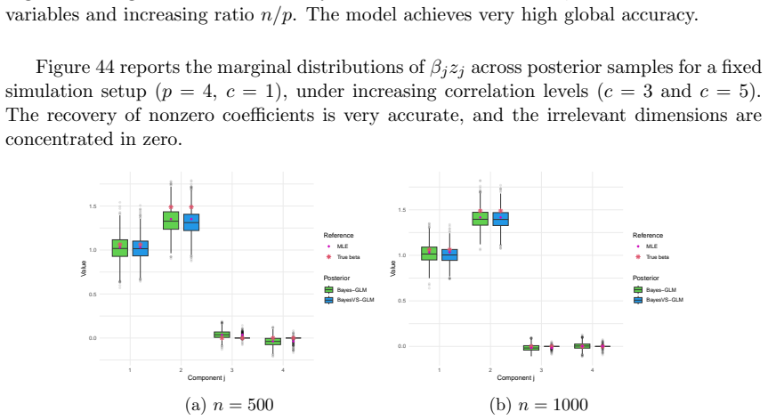
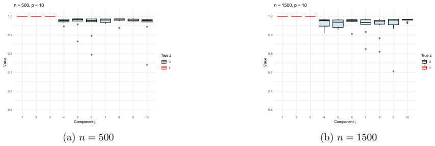
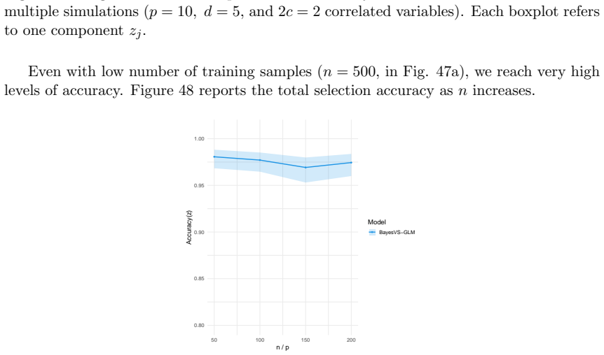
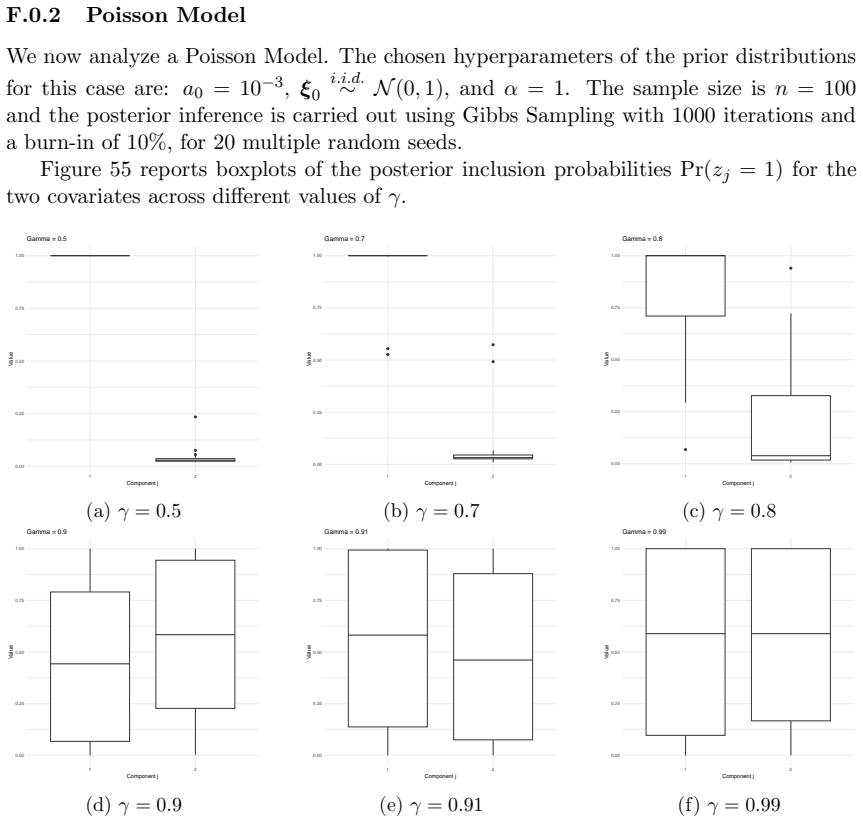
Figures


read the original abstract
Covariate selection in Generalized Linear Models (GLMs) is a fundamental problem in statistics, as including irrelevant predictors might lead to overfitting and poor interpretability, while omitting relevant ones might result in biased estimates. Most Bayesian approaches to variable selection -- including spike-and-slab priors and continuous shrinkage priors -- have key limitations, e.g., (i) are based on non fully conjugate formulations, (ii) are restricted to a linear model, or (iii) lack posterior consistency guarantees for the variable selection procedure and model parameters. In this work, we propose a fully Bayesian hierarchical and conjugate framework for covariate selection in GLMs, applicable to any distribution in the exponential family, based on modeling a binary inclusion indicator that directly encodes covariate inclusion in the linear predictor. In our approach, variable selection and parameter estimation are performed simultaneously, incorporating both sources of uncertainty in posterior inference. Consequently, our methodology provides a valid post-model Bayesian selection procedure. We present theoretical guarantees of the proposed fully conjugate Bayesian variable selection for GLMs, establishing posterior consistency of both the inclusion indicators and the active regression coefficients. We derive an efficient Gibbs Sampling algorithm with a corresponding R package implementation. We validate the proposed method on synthetic and real-world datasets, demonstrating competitive predictive and inferential performance.
Editorial analysis
A structured set of objections, weighed in public.
Referee Report
Summary. The manuscript proposes a fully Bayesian hierarchical and conjugate framework for covariate selection in generalized linear models (GLMs) applicable to any exponential-family distribution. It models binary inclusion indicators that directly encode covariate inclusion in the linear predictor, enabling simultaneous variable selection and parameter estimation via a Gibbs sampler (with R package). The central claims are posterior consistency of the inclusion indicators and active regression coefficients, along with competitive performance on synthetic and real data.
Significance. If the conjugacy construction and consistency results hold, the work would address documented limitations of existing spike-and-slab and shrinkage approaches (non-conjugacy, restriction to linear models, lack of selection consistency) by supplying a broadly applicable conjugate formulation with explicit posterior-consistency guarantees. The open R implementation would further support reproducibility.
major comments (2)
- [§3] §3 (theoretical results): the abstract asserts posterior consistency for both inclusion indicators and active coefficients, yet the provided text contains no proof sketch, no statement of the required assumptions on the design matrix or link function, and no reference to the specific theorem establishing the result. Without these details the load-bearing claim cannot be verified.
- [§4] §4 (Gibbs sampler): the claim of a 'fully conjugate' hierarchical model for arbitrary exponential-family GLMs is central, but the text supplies neither the explicit full-conditional derivations nor the form of the prior on the inclusion indicators that would be needed to confirm conjugacy holds beyond the Gaussian case.
minor comments (2)
- The abstract states that the method 'provides a valid post-model Bayesian selection procedure,' but the manuscript does not clarify how the joint posterior is used for selection versus the usual marginal inclusion probabilities.
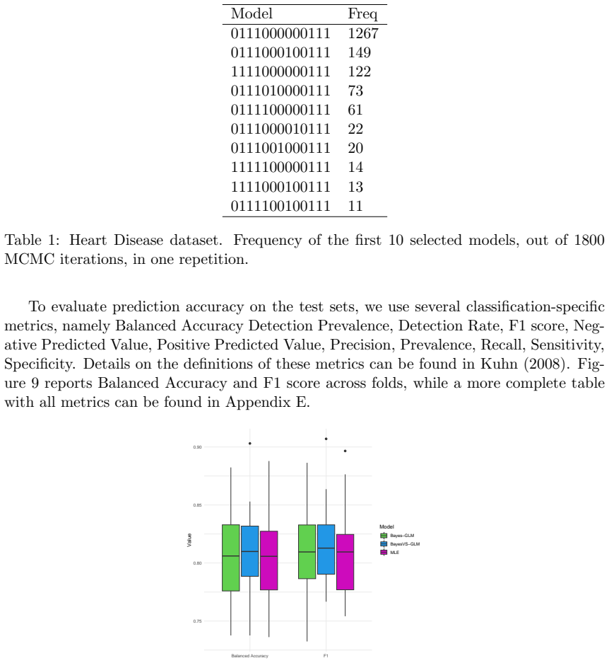
- Table and figure captions should explicitly state the GLM family, link function, and sample size used in each experiment so that the synthetic-data results can be reproduced from the description alone.
Simulated Author's Rebuttal
We thank the referee for their constructive comments on our manuscript. We address each of the major comments below, indicating the revisions we will make to improve clarity and completeness.
read point-by-point responses
-
Referee: [§3] §3 (theoretical results): the abstract asserts posterior consistency for both inclusion indicators and active coefficients, yet the provided text contains no proof sketch, no statement of the required assumptions on the design matrix or link function, and no reference to the specific theorem establishing the result. Without these details the load-bearing claim cannot be verified.
Authors: The referee is correct that the current manuscript version does not include a proof sketch or explicit assumptions in the main text. We will revise the manuscript to include a dedicated subsection in §3 with a proof sketch, a clear statement of the assumptions (including conditions on the design matrix such as bounded eigenvalues and on the link function for the exponential family), and a reference to the theorem number. This will allow verification of the posterior consistency claims for the inclusion indicators and active coefficients. revision: yes
-
Referee: [§4] §4 (Gibbs sampler): the claim of a 'fully conjugate' hierarchical model for arbitrary exponential-family GLMs is central, but the text supplies neither the explicit full-conditional derivations nor the form of the prior on the inclusion indicators that would be needed to confirm conjugacy holds beyond the Gaussian case.
Authors: We agree that explicit derivations are necessary to substantiate the conjugacy claim for general GLMs. In the revision, we will add an appendix containing the full-conditional distributions for all parameters, including the derivation steps, and specify the prior on the inclusion indicators (a product of independent Bernoulli distributions with success probability depending on a hyperparameter). This will demonstrate how conjugacy is achieved for arbitrary exponential-family distributions via the hierarchical structure. revision: yes
Circularity Check
No significant circularity identified
full rationale
The abstract and provided material present a new hierarchical model using binary inclusion indicators to achieve conjugacy for any exponential-family GLM, with separate posterior consistency results for inclusions and coefficients. No equations or steps are shown that reduce by construction to fitted inputs, self-definitions, or load-bearing self-citations; the consistency claims are stated as independent theoretical guarantees rather than re-expressions of the model inputs. The derivation chain is therefore self-contained against external benchmarks.
Axiom & Free-Parameter Ledger
axioms (1)
- domain assumption The response distribution belongs to the exponential family.
Reference graph
Works this paper leans on
-
[1]
Alan Agresti. Categorical Data Analysis. John Wiley & Sons, 2002. doi:10.1002/0471249688
-
[2]
Charalambos D Aliprantis and Kim C Border. Infinite Dimensional Analysis: A Hitchhiker's Guide. Springer, 2006. doi:10.1007/3-540-29587-9
-
[3]
Multivariate exponential families: a concise guide to statistical inference
Stefan Bedbur and Udo Kamps. Multivariate exponential families: a concise guide to statistical inference. Springer, 2021. doi:10.1007/978-3-030-81900-2
-
[4]
Lasso meets horseshoe
Anindya Bhadra, Jyotishka Datta, Nicholas G Polson, and Brandon Willard. Lasso meets horseshoe. Statistical Science, 34 0 (3): 0 405--427, 2019
2019
-
[5]
The horseshoe-like regularization for feature subset selection
Anindya Bhadra, Jyotishka Datta, Nicholas G Polson, and Brandon T Willard. The horseshoe-like regularization for feature subset selection. Sankhy \=a : The Indian Journal of Statistics, Series B , 83 0 (1): 0 185--214, 2021
2021
-
[6]
Fast empirical bayesian lasso for multiple quantitative trait locus mapping
Xiaodong Cai, Anhui Huang, and Shizhong Xu. Fast empirical bayesian lasso for multiple quantitative trait locus mapping. BMC bioinformatics, 12: 0 1--13, 2011
2011
-
[7]
Bayesian inference on hierarchical nonlocal priors in generalized linear models
Xuan Cao and Kyoungjae Lee. Bayesian inference on hierarchical nonlocal priors in generalized linear models. Bayesian Analysis, 19 0 (1): 0 99--122, 2024
2024
-
[8]
High-dimensional sparse factor modeling: applications in gene expression genomics
Carlos M Carvalho, Jeffrey Chang, Joseph E Lucas, Joseph R Nevins, Quanli Wang, and Mike West. High-dimensional sparse factor modeling: applications in gene expression genomics. Journal of the American Statistical Association, 103 0 (484): 0 1438--1456, 2008
2008
-
[9]
Conjugate priors for generalized linear models
Ming-Hui Chen and Joseph G Ibrahim. Conjugate priors for generalized linear models. Statistica Sinica, 13 0 (2): 0 461--476, 2003
2003
-
[10]
Bayesian variable selection and computation for generalized linear models with conjugate priors
Ming-Hui Chen, Lan Huang, Joseph G Ibrahim, and Sungduk Kim. Bayesian variable selection and computation for generalized linear models with conjugate priors. Bayesian analysis (Online), 3 0 (3): 0 585, 2008
2008
-
[11]
On bayesian model and variable selection using mcmc
Petros Dellaportas, Jonathan J Forster, and Ioannis Ntzoufras. On bayesian model and variable selection using mcmc. Statistics and computing, 12 0 (1): 0 27--36, 2002
2002
-
[12]
Conjugate priors for exponential families
Persi Diaconis and Donald Ylvisaker. Conjugate priors for exponential families. Annals of Statistics, 7: 0 269--281, 1979
1979
-
[13]
Ideal spatial adaptation by wavelet shrinkage
David L Donoho and Iain M Johnstone. Ideal spatial adaptation by wavelet shrinkage. biometrika, 81 0 (3): 0 425--455, 1994
1994
-
[14]
Variable selection via nonconcave penalized likelihood and its oracle properties
Jianqing Fan and Runze Li. Variable selection via nonconcave penalized likelihood and its oracle properties. Journal of the American statistical Association, 96 0 (456): 0 1348--1360, 2001
2001
-
[15]
A statistical view of some chemometrics regression tools
LLdiko E Frank and Jerome H Friedman. A statistical view of some chemometrics regression tools. Technometrics, 35 0 (2): 0 109--135, 1993
1993
-
[16]
Penalized regressions: the bridge versus the lasso
Wenjiang J Fu. Penalized regressions: the bridge versus the lasso. Journal of computational and graphical statistics, 7 0 (3): 0 397--416, 1998
1998
-
[17]
Identifiability, improper priors, and gibbs sampling for generalized linear models
Alan E Gelfand and Sujit K Sahu. Identifiability, improper priors, and gibbs sampling for generalized linear models. Journal of the American Statistical Association, 94 0 (445): 0 247--253, 1999
1999
-
[18]
Bayesian data analysis
Andrew Gelman, John B Carlin, Hal S Stern, and Donald B Rubin. Bayesian data analysis. Chapman and Hall/CRC, 1995
1995
-
[19]
Variable selection via gibbs sampling
Edward I George and Robert E McCulloch. Variable selection via gibbs sampling. Journal of the American Statistical Association, 88 0 (423): 0 881--889, 1993
1993
-
[20]
An Introduction to Bayesian Analysis: Theory and Methods
Jayanta K Ghosh, Mohan Delampady, and Tapas Samanta. An Introduction to Bayesian Analysis: Theory and Methods. Springer, 2007
2007
-
[21]
Spike and slab variable selection: Frequentist and bayesian strategies
Hemant Ishwaran and J Sunil Rao. Spike and slab variable selection: Frequentist and bayesian strategies. Annals of Statistics, 33 0 (2): 0 730--773, 2005
2005
-
[22]
Heart disease dataset
Andras Janosi, William Steinbrunn, Matthias Pfisterer, and Robert Detrano. Heart disease dataset. UCI Machine Learning Repository, 1988. Data collected at: Hungarian Institute of Cardiology (Budapest); University Hospital, Zurich, Switzerland; University Hospital, Basel, Switzerland; V.A. Medical Center, Long Beach and Cleveland Clinic Foundation. Availab...
1988
-
[23]
On the use of non-local prior densities in bayesian hypothesis tests
Valen E Johnson and David Rossell. On the use of non-local prior densities in bayesian hypothesis tests. Journal of the Royal Statistical Society Series B: Statistical Methodology, 72 0 (2): 0 143--170, 2010
2010
-
[24]
Bayesian model selection in high-dimensional settings
Valen E Johnson and David Rossell. Bayesian model selection in high-dimensional settings. Journal of the American Statistical Association, 107 0 (498): 0 649--660, 2012
2012
-
[25]
Robust linear model selection based on least angle regression
Jafar A Khan, Stefan Van Aelst, and Ruben H Zamar. Robust linear model selection based on least angle regression. Journal of the American Statistical Association, 102 0 (480): 0 1289--1299, 2007
2007
-
[26]
Building predictive models in R using the caret package
Max Kuhn. Building predictive models in R using the caret package. Journal of Statistical Software, 28 0 (5): 0 1–26, 2008. doi:10.18637/jss.v028.i05
-
[27]
Variable selection for regression models
Lynn Kuo and Bani Mallick. Variable selection for regression models. Sankhy \=a : The Indian Journal of Statistics, Series B , 60 0 (1): 0 65--81, 1998
1998
-
[28]
Bayesian group selection in logistic regression with application to mri data analysis
Kyoungjae Lee and Xuan Cao. Bayesian group selection in logistic regression with application to mri data analysis. Biometrics, 77 0 (2): 0 391--400, 2021
2021
-
[29]
Mixtures of g priors for bayesian variable selection
Feng Liang, Rui Paulo, German Molina, Merlise A Clyde, and Jim O Berger. Mixtures of g priors for bayesian variable selection. Journal of the American Statistical Association, 103 0 (481): 0 410--423, 2008
2008
-
[30]
Bayesian approaches to variable selection: a comparative study from practical perspectives
Zihang Lu and Wendy Lou. Bayesian approaches to variable selection: a comparative study from practical perspectives. The International Journal of Biostatistics, 18 0 (1): 0 83--108, 2022. doi:10.1515/ijb-2020-0130
-
[31]
Sparse statistical modelling in gene expression genomics
Joe Lucas, Carlos Carvalho, Quanli Wang, Andrea Bild, Joseph R Nevins, and Mike West. Sparse statistical modelling in gene expression genomics. Bayesian inference for gene expression and proteomics, 1 0 (1): 0 1644, 2006
2006
-
[32]
Comparing spike and slab priors for bayesian variable selection
Gertraud Malsiner-Walli and Helga Wagner. Comparing spike and slab priors for bayesian variable selection. Austrian Journal of Statistics, 40 0 (4), 2016
2016
-
[33]
Instabilities of regression estimates relating air pollution to mortality
Gary C McDonald and Richard C Schwing. Instabilities of regression estimates relating air pollution to mortality. Technometrics, 15 0 (3): 0 463--481, 1973
1973
-
[34]
Asymptotic normality, concentration, and coverage of generalized posteriors
Jeffrey W Miller. Asymptotic normality, concentration, and coverage of generalized posteriors. Journal of Machine Learning Research, 22 0 (168): 0 1--53, 2021
2021
-
[35]
Bayesian variable selection in linear regression
Toby J Mitchell and John J Beauchamp. Bayesian variable selection in linear regression. Journal of the American Statistical Association, 83 0 (404): 0 1023--1032, 1988
1988
-
[36]
Bayesian variable selection with shrinking and diffusing priors
Naveen N Narisetty and Xuming He. Bayesian variable selection with shrinking and diffusing priors. Annals of Statistics, 42 0 (2): 0 789--817, 2014
2014
-
[37]
Journal of the American Statistical Association , author =
Naveen N Narisetty, Juan Shen, and Xuming He. Skinny gibbs: A consistent and scalable gibbs sampler for model selection. Journal of the American Statistical Association, 114 0 (527): 0 1205--1217, 2019. doi:10.1080/01621459.2018.1482754
-
[38]
Flamby: Datasets and benchmarks for cross-silo federated learning in realistic healthcare settings
Jean Ogier du Terrail, Samy-Safwan Ayed, Edwige Cyffers, Felix Grimberg, Chaoyang He, Regis Loeb, Paul Mangold, Tanguy Marchand, Othmane Marfoq, Erum Mushtaq, et al. Flamby: Datasets and benchmarks for cross-silo federated learning in realistic healthcare settings. Advances in Neural Information Processing Systems, 35: 0 5315--5334, 2022
2022
-
[39]
Robert B O'hara and Mikko J Sillanp \"a \"a . A review of Bayesian variable selection methods: what, how and which . Bayesian Analysis, 4 0 (1): 0 85 -- 117, 2009. doi:10.1214/09-BA403
-
[40]
Mario Padilla Rodriguez and Mohamed Nafea. Centralized and federated heart disease classification models using uci dataset and their shapley-value based interpretability, 2024. URL https://arxiv.org/abs/2408.06183
arXiv 2024
-
[41]
High-dimensional bayesian classifiers using non-local priors
David Rossell, Donatello Telesca, and Valen E Johnson. High-dimensional bayesian classifiers using non-local priors. In Statistical models for data analysis, pages 305--313. Springer, 2013
2013
-
[42]
Hanson-wright inequality and sub-gaussian concentration
Mark Rudelson and Roman Vershynin. Hanson-wright inequality and sub-gaussian concentration. Electronic Communications in Probability, 18, 2013. doi:10.1214/ECP.v18-2865
-
[43]
Some notes on concentration for -subexponential random variables
Holger Sambale. Some notes on concentration for -subexponential random variables. In Rados aw Adamczak, Nathael Gozlan, Karim Lounici, and Mokshay Madiman, editors, High Dimensional Probability IX, pages 167--192. Springer International Publishing, 2023. doi:10.1007/978-3-031-26979-0\_7
-
[44]
Scalable bayesian variable selection using nonlocal prior densities in ultrahigh-dimensional settings
Minsuk Shin, Anirban Bhattacharya, and Valen E Johnson. Scalable bayesian variable selection using nonlocal prior densities in ultrahigh-dimensional settings. Statistica Sinica, 28 0 (2): 0 1053, 2018
2018
-
[45]
Optimizing heart disease diagnosis with advanced machine learning models: a comparison of predictive performance
M Darshan Teja and G Mokesj Rayalu. Optimizing heart disease diagnosis with advanced machine learning models: a comparison of predictive performance. BMC Cardiovascular Disorders, 25 0 (1): 0 212, 2025
2025
-
[46]
Regression shrinkage and selection via the lasso
Robert Tibshirani. Regression shrinkage and selection via the lasso. Journal of the Royal Statistical Society. Series B (Methodological), 58 0 (1): 0 267--288, 1996
1996
-
[47]
On the existence and uniqueness of the maximum likelihood estimates for certain generalized linear models
Robert WM Wedderburn. On the existence and uniqueness of the maximum likelihood estimates for certain generalized linear models. Biometrika, 63 0 (1): 0 27--32, 1976
1976
-
[48]
Mike West. Bayesian factor regression models in the “large p , small n ” paradigm. Bayesian statistics, 7: 0 733--742, 2003. doi:10.1093/oso/9780198526155.003.0053
-
[49]
Nonlocal Priors in Generalized Linear Models and Gaussian Graphical Models
Fang Yang. Nonlocal Priors in Generalized Linear Models and Gaussian Graphical Models. PhD thesis, University of Cincinnati, 2022. URL http://rave.ohiolink.edu/etdc/view?acc_num=ucin1659529506044173,
2022
discussion (0)
Sign in with ORCID, Apple, or X to comment. Anyone can read and Pith papers without signing in.