Data-Driven Duration Management -- Term Structure Forecasting Using Machine Learning
Pith reviewed 2026-06-26 01:48 UTC · model grok-4.3
The pith
Neural networks that integrate factor models outperform classical econometric approaches in forecasting U.S. and European government bond yield curves.
A machine-rendered reading of the paper's core claim, the machinery that carries it, and where it could break.
Core claim
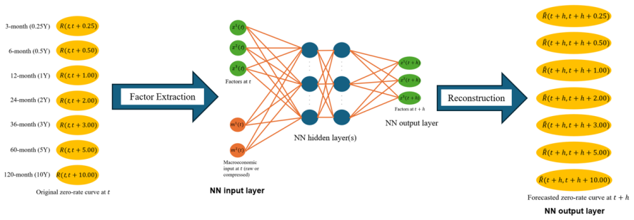
Neural networks consistently outperform traditional models in both forecasting accuracy and portfolio performance. For the U.S., the most effective approach is a direct-forecasting NN that incorporates DNS factors to reduce the dimensionality of zero-rate data and an Autoencoder to extract macroeconomic features, while for Europe, the optimal model is a factor-based NN using PCA-derived zero-rate factors without the integration of macroeconomic variables.
What carries the argument
Neural network architectures that blend classical factor models like DNS and PCA with machine learning techniques for dimensionality reduction and feature extraction.
If this is right
- Neural networks improve both statistical forecasting accuracy and the returns from quantitative bond trading strategies.
- Different optimal model configurations apply to the U.S. Treasury market versus the European market.
- Macroeconomic variables enhance neural network performance in the U.S. but are not beneficial in Europe.
- Combining traditional term structure models with modern machine learning supports better fixed-income portfolio construction.
Where Pith is reading between the lines
- These findings could support more effective duration management in bond portfolios by providing better yield curve forecasts.
- Similar machine learning approaches might be tested on corporate bonds or other fixed-income assets.
- The model evaluation framework combining statistical and economic metrics could be applied to other forecasting problems in finance.
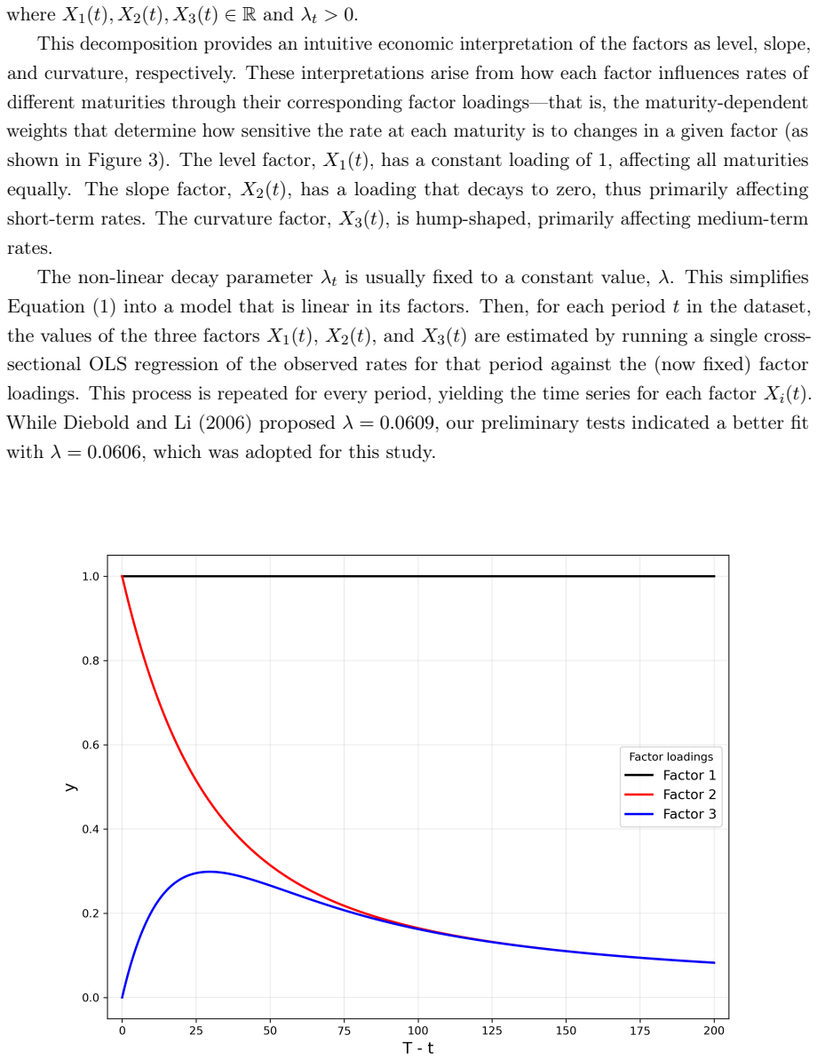
Load-bearing premise
The reported outperformance reflects genuine predictive power rather than overfitting to the specific sample periods or data choices, and the quantitative trading strategy evaluation accurately captures economic value without look-ahead bias.
What would settle it
Re-running the analysis on data from a subsequent period not included in the original sample to check if the neural network models maintain their advantage in forecasting accuracy and trading performance.
Figures


read the original abstract
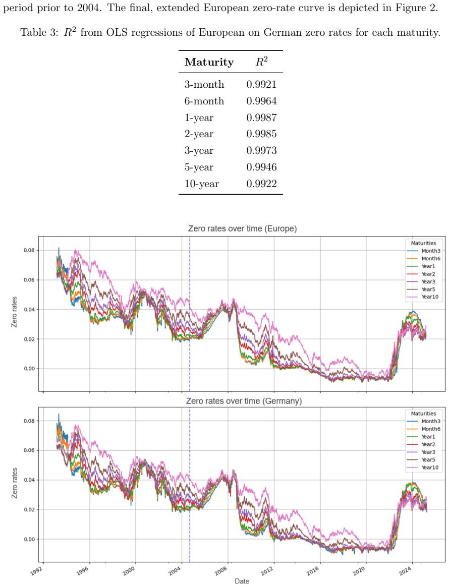
This paper compares different methods for forecasting the term structure of U.S. and European zero-coupon government bonds using both traditional econometric and Machine Learning (ML) approaches. We compare classical models (e.g., Dynamic Nelson-Siegel (DNS) and Principal Component Analysis (PCA)) with different Neural Network (NN) architectures, including those inspired by the classical models, on the U.S. Treasury market and bonds issued by the European Central Bank (ECB). To enhance predictive performance, macroeconomic variables are incorporated. The findings for both markets are separately analyzed and compared. To this end, we propose a robust model evaluation framework combining statistical accuracy metrics - such as RMSE, MAE, and directional accuracy - with the economic relevance of a quantitative bond trading strategy. Results show that NNs consistently outperform traditional models in both forecasting accuracy and portfolio performance. For the U.S., the most effective approach is a direct-forecasting NN that incorporates DNS factors to reduce the dimensionality of zero-rate data and an Autoencoder (AE) to extract macroeconomic features, while for Europe, the optimal model is a factor-based NN using PCA-derived zero-rate factors without the integration of macroeconomic variables. Overall, the paper demonstrates how combining traditional modeling approaches with modern ML techniques and evaluation can improve yield curve forecasts and support applications in fixed-income portfolio construction.
Editorial analysis
A structured set of objections, weighed in public.
Referee Report
Summary. The paper compares classical term structure models (Dynamic Nelson-Siegel and PCA) against multiple neural network architectures for forecasting US Treasury and ECB zero-coupon yields. Macroeconomic variables are added as inputs. Models are assessed via RMSE, MAE, directional accuracy, and the economic performance of a quantitative bond trading strategy. The central claim is that NNs consistently outperform the baselines, with a direct-forecasting NN (DNS factors + autoencoder for macros) optimal for the US and a factor-based NN (PCA zero-rate factors, no macros) optimal for Europe.
Significance. If the outperformance survives rigorous out-of-sample validation and controls for data snooping, the integration of classical factor structures with ML could improve yield-curve forecasting and fixed-income portfolio construction. The dual statistical-plus-economic evaluation metric is a constructive feature.
major comments (2)
- [Abstract] Abstract and evaluation framework: the manuscript asserts a 'robust model evaluation framework' yet supplies no concrete description of cross-validation, walk-forward hyperparameter selection, fixed training windows, or adjustments for multiple testing across architectures, factor choices, and macro inclusions. This is load-bearing for the claim of consistent NN superiority, as the results remain vulnerable to overfitting and look-ahead bias.
- [Evaluation framework] Trading-strategy evaluation: because portfolio returns are computed directly from the forecasts, the paper must demonstrate that the strategy metric is free of look-ahead bias and that any hyperparameter tuning for the NNs was performed without using information from the evaluation period.
Simulated Author's Rebuttal
We thank the referee for highlighting the need for greater transparency in our evaluation procedures. We agree that explicit documentation of cross-validation, walk-forward selection, and bias controls is essential to support the robustness claims. Below we address each major comment and commit to expanding the relevant sections in revision.
read point-by-point responses
-
Referee: [Abstract] Abstract and evaluation framework: the manuscript asserts a 'robust model evaluation framework' yet supplies no concrete description of cross-validation, walk-forward hyperparameter selection, fixed training windows, or adjustments for multiple testing across architectures, factor choices, and macro inclusions. This is load-bearing for the claim of consistent NN superiority, as the results remain vulnerable to overfitting and look-ahead bias.
Authors: We acknowledge that the current manuscript provides only a high-level reference to the evaluation framework without sufficient procedural detail. In the revised version we will add a dedicated subsection that specifies: (i) a rolling walk-forward scheme with fixed-length training windows ending at each forecast origin, (ii) hyperparameter selection performed exclusively via inner cross-validation on the training window (no test-period information), and (iii) a Bonferroni-style adjustment for the finite set of architectures and macro inclusions examined. These additions will be placed in both the methodology and results sections. revision: yes
-
Referee: [Evaluation framework] Trading-strategy evaluation: because portfolio returns are computed directly from the forecasts, the paper must demonstrate that the strategy metric is free of look-ahead bias and that any hyperparameter tuning for the NNs was performed without using information from the evaluation period.
Authors: We agree that explicit safeguards against look-ahead bias in the trading-strategy metric are required. The revised manuscript will include a new paragraph in the economic-evaluation section stating that (a) all positions are formed using only forecasts generated from models trained up to the rebalancing date, (b) transaction costs and slippage are applied at the subsequent period's realized prices, and (c) hyperparameter grids were optimized solely on the in-sample training folds with no leakage from the out-of-sample evaluation window. We will also report the exact training-window lengths and rebalancing frequency used. revision: yes
Circularity Check
No significant circularity detected
full rationale
The paper performs an empirical out-of-sample comparison of NN architectures against DNS and PCA baselines on RMSE/MAE/directional accuracy plus a separate quantitative bond trading strategy whose returns are computed from the forecasts. No equations, derivations, or self-citations are shown that reduce any claimed prediction or uniqueness result to a fitted input or prior author work by construction. The evaluation metrics and trading performance are independent of the model-fitting objective, satisfying the default expectation of a non-circular empirical study.
Axiom & Free-Parameter Ledger
Reference graph
Works this paper leans on
-
[1]
doi: 10.1016/S0304-3932(03)00032-1. Pierre Baldi and Kurt Hornik. Neural networks and principal component analysis: Learning from examples without local minima.Neural networks, 2(1):53–58,
-
[2]
Wei Bao, Jun Yue, and Yulei Rao
doi: 10.1016/0893-6080(89) 90014-2. Wei Bao, Jun Yue, and Yulei Rao. A deep learning framework for financial time series using stacked autoencoders and long-short term memory.PLOS ONE, 12(7):e0180944,
-
[3]
doi: 10.1371/journal.pone.0180944. Christoph Bergmeir, José M. Benítez, and Fivos Malliaros. A note on the accuracy of cross- validation for evaluating time series forecasting methods.Journal of Forecasting, 37(1):27–41,
-
[4]
doi: 10.1002/for.2505. David Blake, Andrew J. Cairns, and Kevin Dowd. Pension metrics: Stochastic pension plan design and value-at-risk during the accumulation phase.Insurance: Mathematics and Economics, 29 (2):187–215,
-
[5]
Ralf Brüggemann, Helmut Lütkepohl, and Massimiliano Marcellino
doi: 10.1016/S0167-6687(01)00082-8. Ralf Brüggemann, Helmut Lütkepohl, and Massimiliano Marcellino. Forecasting euro area variables with german pre-emu data.Journal of Forecasting, 27(6):465–481,
-
[6]
Alexei Chekhlov, Stanislav Uryasev, and Michael Zabarankin
doi: 10.1002/for.1064. Alexei Chekhlov, Stanislav Uryasev, and Michael Zabarankin. Drawdown measure in portfolio optimization.International Journal of Theoretical and Applied Finance, 8(01):13–58,
-
[7]
Jens HE Christensen, Francis X Diebold, and Glenn D Rudebusch
doi: 10.1142/S0219024905002767. Jens HE Christensen, Francis X Diebold, and Glenn D Rudebusch. The affine arbitrage-free class of nelson–siegel term structure models.Journal of Econometrics, 164(1):4–20,
-
[8]
doi: 10.1016/j.jeconom.2011.03.015. Todd E. Clark. Do producer prices lead consumer prices?Federal Reserve Bank of Kansas City Economic Review, 80(3):25–39,
-
[9]
John H Cochrane and Monika Piazzesi
URLhttps://www.kansascityfed.org/documents/ 1005/1995-Do%20Producer%20Prices%20Lead%20Consumer%20Prices%3F.pdf. John H Cochrane and Monika Piazzesi. Bond risk premia.American Economic Review, 95(1): 138–160,
1995
-
[10]
Francis X Diebold and Canlin Li
doi: 10.1257/0002828053828581. Francis X Diebold and Canlin Li. Forecasting the term structure of government bond yields. Journal of Econometrics, 130(2):337–364,
-
[11]
Christian L Dunis and Vincent Morrison
doi: 10.1016/j.jeconom.2005.03.005. Christian L Dunis and Vincent Morrison. The economic value of advanced time series methods for modelling and trading 10-year government bonds.European Journal of Finance, 13(4): 333–352,
-
[12]
37 Janina Engel, Markus Wahl, and Rudi Zagst
doi: 10.1080/13518470600880010. 37 Janina Engel, Markus Wahl, and Rudi Zagst. Forecasting turbulence in the asian and european stock market using regime-switching models.Quantitative Finance and Economics, 2(2): 388–406,
-
[13]
Frank J Fabozzi.Fixed Income Analysis
doi: 10.3934/QFE.2018.2.388. Frank J Fabozzi.Fixed Income Analysis. John Wiley & Sons,
-
[14]
Stefan Falkner, Aaron Klein, and Frank Hutter
doi: 10.1002/9781119197368. Stefan Falkner, Aaron Klein, and Frank Hutter. BOHB: Robust and efficient hyperparameter optimization at scale. InInternational Conference on Machine Learning, volume 80 of Proceedings of Machine Learning Research, pages 1437–1446. PMLR,
-
[15]
URL http: //proceedings.mlr.press/v80/falkner18a.html. Solveig Flaig and Gero Junike. Validation of machine learning based scenario generators.arXiv preprint arXiv:2301.12719,
-
[16]
doi: 10.48550/arXiv.2301.12719. Johnny Kang and Carolin E. Pflueger. Inflation risk in corporate bonds.The Journal of Finance, 70(1):115–162,
-
[17]
URLhttps://onlinelibrary.wiley.com/doi/ abs/10.1111/jofi.12195
doi: 10.1111/jofi.12195. URLhttps://onlinelibrary.wiley.com/doi/ abs/10.1111/jofi.12195. Con Keating and William F Shadwick. A universal performance measure.The Finance De- velopment Centre,
-
[18]
Available at SSRN:https://ssrn.com/ abstract=1110463
doi: 10.2139/ssrn.1110463. Available at SSRN:https://ssrn.com/ abstract=1110463. Tae Yoon Kim, Kyong Joo Oh, Chiho Kim, and Jong Doo Do. Artificial neural networks for non- stationary time series.Neurocomputing, 61:439–447,
-
[19]
Charles R Nelson and Andrew F Siegel
doi: 10.1016/j.neucom.2004.04.002. Charles R Nelson and Andrew F Siegel. Parsimonious modeling of yield curves.The Journal of Business, 60(4):473–489,
-
[20]
Manuel Nunes, Enrico Gerding, Frank McGroarty, and Mahesan Niranjan
doi: 10.1086/296409. Manuel Nunes, Enrico Gerding, Frank McGroarty, and Mahesan Niranjan. A comparison of multitask and single task learning with artificial neural networks for yield curve forecasting. Expert Systems with Applications, 119:362–375,
-
[21]
Evangelos Salachas, Georgios P Kouretas, and Nikiforos T Laopodis
doi: 10.1016/j.eswa.2018.11.012. Evangelos Salachas, Georgios P Kouretas, and Nikiforos T Laopodis. The term structure of interest rates and economic activity: Evidence from the covid-19 pandemic.Journal of Forecasting, 43(4):1018–1041,
-
[22]
Yoshiyuki Suimon, Hiroki Sakaji, Kiyoshi Izumi, and Hiroyasu Matsushima
doi: 10.1002/for.3082. Yoshiyuki Suimon, Hiroki Sakaji, Kiyoshi Izumi, and Hiroyasu Matsushima. Autoencoder-based three-factor model for the yield curve of japanese government bonds and a trading strategy. Journal of Risk and Financial Management, 13(4):82,
-
[23]
doi: 10.3390/jrfm13040082. Leonard J Tashman. Out-of-sample tests of forecasting accuracy: an analysis and review. International Journal of Forecasting, 16(4):437–450,
-
[24]
doi: 10.1016/S0169-2070(00)00065-0. Daniel Vela. Forecasting latin-american yield curves: An artificial neural network approach.Bor- radores de Economía, (761),
-
[25]
doi: 10.1007/ 978-3-662-09950-8. 38 1 Supplementary Document: Data-Driven Duration Management 1 Optimized Hyperparameters for the NNs Table 1.1: Optimized hyperparameters for the models presented in Table A1 of the paper with U.S. data. Here we test different values for the number of training epochs. In some cases, model performance improved when the numb...
2000
-
[26]
In some cases, model performance improved when the number of training epochs was reduced from 2000 to
Model Learning Rate Activation Function Batch Size Number of Lay- ers Neurons in Layer 1 Neurons in Layer 2 Epochs 8 0.001530 tanh 54 1 6 0 2000 9 0.005330 ReLu 30 1 4 0 2000 10 0.004675 ReLu 26 1 5 0 2000 11 0.002496 tanh 27 2 3 4 2000 12 0.001760 tanh 47 2 3 4 2000 13 0.001020 ReLu 59 1 8 0 2000 14 0.036207 ReLu 98 1 3 0 2000 15 0.000555 ReLu 63 1 5 0 1...
2000
-
[27]
Further reductions did not lead to additional gains. Model Learning Rate Activation Function Batch Size Number of Lay- ers Neurons in Layer 1 Neurons in Layer 2 Epochs 8 0.001074 tanh 44 1 6 0 2000 9 0.001450 tanh 90 1 4 0 2000 10 0.000234 tanh 26 2 5 5 2000 11 0.000204 tanh 38 2 3 9 2000 12 0.059644 ReLu 66 2 7 9 2000 13 0.010095 ReLu 38 1 6 0 2000 14 0....
2000
-
[28]
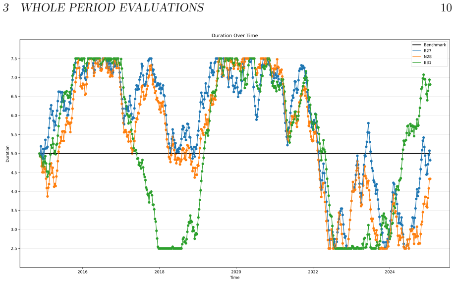
3 WHOLE PERIOD EV ALUATIONS10 Figure 3.2: Duration from the different portfolios between July 2014 and February
2014
-
[29]
3.2 Europe Figure 3.3: Performance from the different models and the benchmark between December 2014 and February
2014
-
[30]
4 PERIODIC EV ALUATION - U.S.11 Figure 3.4: Duration from the different portfolios in Europe between December 2014 and February
2014
-
[31]
Table 4.1: Results for the different models in the period between July 2014 and February
2014
-
[32]
Ω MDD Rank
Model Ret. Ω MDD Rank. Ω Rank. MDD Sum Rank. Rank. P1 B27 0.78 0.95 -7.21 2 2 4 1 N28 0.77 0.93 -7.17 3 1 4 1 B31 1.36 1.06 -7.37 1 3 4 1 Bench. 0.98 - -4.92 - - - - 4 PERIODIC EV ALUATION - U.S.12 Figure 4.1: Performance of the different portfolios between July 2014 and February
2014
-
[33]
Figure 4.2: Duration of the different portfolios between July 2014 and February
2014
-
[34]
4 PERIODIC EV ALUATION - U.S.13 Table 4.2: Results for the different models in the period between February 2018 and July
2018
-
[35]
Figure 4.3: Performance of the different portfolios between February 2018 and July
2018
-
[36]
4 PERIODIC EV ALUATION - U.S.14 Figure 4.4: Duration of the different portfolios between February 2018 and July
2018
-
[37]
Table 4.3: Results for the different models in the period between July 2021 and November
2021
-
[38]
Ω MDD Rank
Model Ret. Ω MDD Rank. Ω Rank. MDD Sum Rank. Rank. P3 B27 -6.48 1.43 -9.51 3 3 6 3 N28 -5.96 1.58 -8.73 1 1 2 1 B31 -6.43 1.49 -9.32 2 2 4 2 Bench. -8.02 - -11.50 - - - - 4 PERIODIC EV ALUATION - U.S.15 Figure 4.5: Performance of the different portfolios between July 2021 and November
2021
-
[39]
Figure 4.6: Duration of the different portfolios between July 2021 and November
2021
-
[40]
4 PERIODIC EV ALUATION - U.S.16 Table 4.4: Results for the different models in the period between November 2022 and February
2022
-
[41]
Figure 4.7: Performance of the different portfolios between November 2022 and February
2022
-
[42]
5 PERIODIC EV ALUATION - EUROPE17 Figure 4.8: Duration of the different portfolios between November 2022 and February
2022
-
[43]
Table 5.1: Results for the different models in the period between December 2014 and September
2014
-
[44]
Ω MDD Rank
Model Ret. Ω MDD Rank. Ω Rank. MDD Sum Rank. Rank. P1 N16 2.26 1.19 -7.60 1 3 4 2 E18 1.64 0.93 -5.49 3 2 5 3 E27 1.85 1.04 -5.09 2 1 3 1 Bench. 1.79 - -5.45 - - - - 5 PERIODIC EV ALUATION - EUROPE18 Figure 5.1: Performance of the different portfolios between December 2014 and September
2014
-
[45]
Figure 5.2: Duration of the different portfolios between December 2014 and September
2014
-
[46]
5 PERIODIC EV ALUATION - EUROPE19 Table 5.2: Results for the different models in the period between September 2019 and November
2019
-
[47]
Figure 5.3: Performance of the different portfolios between September 2019 and November
2019
-
[48]
5 PERIODIC EV ALUATION - EUROPE20 Figure 5.4: Duration of the different portfolios between September 2019 and November
2019
-
[49]
Table 5.3: Results for the different models in the period between December 2021 and October
2021
-
[50]
Ω MDD Rank
Model Ret. Ω MDD Rank. Ω Rank. MDD Sum Rank. Rank. P3 N16 -3.69 1.89 -7.57 1 3 4 1 E18 -3.14 1.88 -7.47 2 2 4 1 E27 -2.50 1.78 -6.53 3 1 4 1 Bench. -6.55 - -12.52 - - - - 5 PERIODIC EV ALUATION - EUROPE21 Figure 5.5: Performance of the different portfolios between December 2021 and October
2021
-
[51]
Figure 5.6: Duration of the different portfolios between December 2021 and October
2021
-
[52]
5 PERIODIC EV ALUATION - EUROPE22 Table 5.4: Results for the different models in the period between October 2023 and Febru- ary
2023
-
[53]
Figure 5.7: Performance of the different portfolios between October 2023 and February
2023
-
[54]
5 PERIODIC EV ALUATION - EUROPE23 Figure 5.8: Duration of the different portfolios between October 2023 and February 2025
2023
discussion (0)
Sign in with ORCID, Apple, or X to comment. Anyone can read and Pith papers without signing in.