REVIEW 3 major objections 4 minor 74 references
An adaptive split-combine Gaussian mixture filter for nonlinear and multimodal state estimation
T0 review · 3 major / 4 minor · reviewed 2026-08-08 · deepseek-v4-flash
Pith's one-line read A new Gaussian-mixture filter splits particles along the level-set direction, halving variance there by construction and tracking skewed, multimodal state densities better than Kalman-type baselines.
desk verdict A genuinely new variance-halving split for Gaussian mixture filters, backed by solid benchmarks, but the bridge from variance reduction to reduced linearization error is asserted, not proved. read the letter →
The pith
A machine-rendered reading of the paper's core claim, the machinery that carries it, and where it could break.
The reading
What carries the argument
The key machinery is the variance-halving split together with the level-set propagation used for each Gaussian particle. Each particle is propagated by tracking level-set points through a velocity field derived from the Fokker–Planck equation under a local linear approximation, avoiding explicit Jacobian and Laplacian computations. When the local linearity check fails, the particle is split into three along the offending level-set-point direction, with a transformation $T$ constructed so that the split direction is uncorrelated with the other coordinates; the child means and covariances are computed with explicit formulas, so no matrix inverse or numerical optimization is needed. The combine step uses a computable upper bound on KL divergence to decide when two particles can be merged.
What would settle it
A concrete test: run the time-update alone on the Van der Pol oscillator with a strongly curved drift, record whether the relative linearization error (13) for child particles after a split falls below $\epsilon_{\mathrm{threshold}}$; if it stays above threshold across several consecutive splits, the variance-halving guarantee does not control the error that the split criterion targets.
Extended reading notes
Core claim
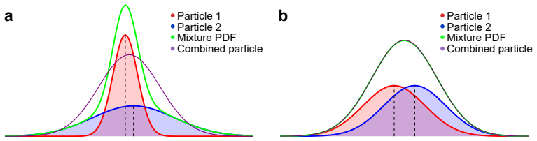
The paper's central discovery is a particle-splitting rule for Gaussian mixtures that reduces variance exactly along a chosen direction rather than along an eigendirection. For a Gaussian with covariance $\Sigma$ and a target unit vector $d$, the child particles have covariance $\Sigma_{\mathrm{split}} = \Sigma - \frac{1}{2} \frac{(\Sigma d)(\Sigma d)^T}{d^T \Sigma d}$, so the variance along $d$ is halved. Because the split is performed in a transformed coordinate system where $d$ is statistically uncorrelated with the remaining directions, the optimal child means and weights from a one-dimensional splitting problem ($a = 1.03332\sigma$, $w = 0.21921$) apply unchanged. The paper argues that splitting along the worst level-set direction reduces the local linearization error that limits Gaussian propagation, without any auxiliary online numerical optimization.
Load-bearing premise
The filter assumes that halving the variance along the worst level-set direction sufficiently reduces the local linearization error, so that level-set propagation of the resulting child particles remains accurate.
Editorial extensions
If this is right
- Filters for highly nonlinear systems with asymmetric and multimodal posteriors can maintain accuracy with far fewer Gaussian particles than the APPD-based approach, reducing computational cost.
- The variance-halving guarantee gives a principled way to target the specific direction that violates local linearity, which prior eigendecomposition-based splits address only indirectly.
- The filter is parallelizable, since particle propagation and splitting are independent across particles, so high-fidelity estimation in chaotic systems becomes practical with CPU-based parallelization.
- The same propagation–split–combine framework applies to pure uncertainty propagation, not only filtering, providing a tool for simulating non-Gaussian density evolution in slow–fast oscillators.
- Weight updates during propagation occur automatically from the split–combine bookkeeping, avoiding auxiliary weight-optimization steps used in earlier Gaussian mixture filters.
Reading between the lines
- The split rule's guarantee could extend to other Gaussian-mixture approximation tasks, such as variational inference or continuous-time generative modeling, wherever a one-dimensional Gaussian split is known to be near-optimal.
- The KL-bound combine rule is a principled alternative to mean-proximity combining and may matter most when components have very different covariances; an ablation comparing AMF's combine rule against mean-proximity combine within the same filter would isolate its contribution.
- The error criterion (13) measures only second- and higher-order drift nonlinearity along a finite set of level-set directions; a natural test is whether splitting along the worst such direction still reduces error when the drift curvature is highly anisotropic or when the threshold $\epsilon_{\mathrm{threshold}}$ is exceeded by many directions at once.
- The claimed accuracy gain over APPDF in the coupled-oscillator case could be probed by replacing only AMF's split rule with APPDF's eigendecomposition split while keeping all other components fixed.
Editorial analysis
A structured set of objections, weighed in public.
Referee Report
Summary. The paper presents AMF, an adaptive split-combine Gaussian mixture filter for continuous-discrete nonlinear state estimation. In the time update, each Gaussian particle is propagated via the level-set method of the level-set Kalman filter; when a relative local-linearization error (Eq. 13) exceeds a threshold, the particle is split into three child particles. The splitting construction is the paper's main theoretical contribution: after a linear transformation that makes the target level-set direction statistically independent of the remaining coordinates, the one-dimensional optimal parameters (a, w) from Eq. (16) are applied, and Theorem 2.1 proves that each child covariance becomes \Sigma - (1/2)\Sigma_\parallel, i.e., the variance along the target direction is halved. Particles are also recombined using a KL-divergence upper bound (Algorithm 3). A measurement update based on the CD-CKF cubature rule and a cubature weight update complete the filter. The method is evaluated on uncertainty propagation and filtering for Van der Pol oscillators, coupled Van der Pol oscillators, and the Lorenz attractor, where it is reported to outperform CD-CKF, LSKF, GS-ACD-ECKF, and APPDF in accuracy while often using fewer particles, and a parallel implementation is described.
Significance. If the algorithmic claims hold, AMF would be a useful addition to the nonlinear filtering toolbox: it avoids online numerical optimization in the splitting step, has a clean geometric variance-halving guarantee (Theorem 2.1), and uses a principled KL-based combining criterion. The experimental section is comparatively careful: PF convergence checks are provided in the supplementary figures, multiple independent runs are reported, and the paper analyzes particle-count dynamics (splits, prunes, combines) to explain why AMF outperforms APPDF. The variance-halving theorem is a genuine and elegant contribution. However, the paper's central accuracy claim goes beyond what is proved: Theorem 2.1 controls the child covariance but does not by itself establish that the local-linearization error (13) falls below \epsilon_{\rm threshold}, and the appendix's identity between the multivariate splitting error and the one-dimensional problem is stated for an L1 error while Eq. (16) is an L-infinity objective. These gaps do not disprove the empirical results, but they leave the theoretical foundation of the adaptive splitting criterion incomplete.
major comments (3)
- [§2.3.2, §2.5, Eq. (13), Theorem 2.1] The splitting criterion and the claimed accuracy gain are not connected by a proof. Theorem 2.1 shows that each child covariance is \Sigma - (1/2)\Sigma_\parallel, which halves the variance along the selected level-set direction. It does not show that the relative error \epsilon in Eq. (13) decreases, either for a single split or after repeated splitting. In Algorithm 2 the two outer child means are displaced by \pm \mu = \pm a\Sigma d_k/(d_k^T\Sigma d_k) (line 12), so the children are not nested in the parent support; their centers can lie in regions where the higher-order drift terms in the numerator of (13) are as large as, or larger than, the parent's. The denominator \|v(\bar{x})\| also changes. The text in §2.3.2 states that splitting 'accelerates satisfaction of the local linear approximation' and §2.5 instructs that splitting be repeated until all particles satisfy the error criterion, but no monotonicity or termination argument is provided. Since the accuracy claim in the abstract ('This enables accurate and efficient propagation') rests on this link, the paper should either provide a quantitative bound showing how \epsilon scales with the reduced column norms and the shift, or explicitly state that the relation between splitting and accuracy is empirical rather than guaranteed.
- [Appendix C and Eq. (16)] The paper states that the error introduced by the splitting procedure is 'identical to the error obtained from the corresponding 1-dimensional particle splitting optimization problem (16)', but the objective in (16) is a min-max (L-infinity) error, whereas Appendix C proves equality only for the L1 error (Eqs. C.4-C.7). The assertion that 'the difference between the errors calculated using the parameter values obtained by solving (16) is negligible (approximately 10^-5)' is not derived and no numerical evidence is given. As written, the claim overstates what is proved. Please correct the statement to refer to the L1 metric or supply the missing computation that connects the L1 and L-infinity errors at the chosen parameters (a,w).
- [Algorithm 2 and Sec. 2.3.2, Eq. (15)] There is a notational mismatch between the motivating optimization problem and the implemented split. Eq. (15) places the outer child means at \pm a u_i, with u_i = x_i/\|x_i\|, i.e., along the level-set direction. The implemented split, by contrast, displaces the children by \pm a\Sigma d/(d^T\Sigma d) (Eq. (26) and Algorithm 2 line 12), which is along \Sigma d and is generally not parallel to d. The reader can infer that (15) is only a one-dimensional motivation and is not solved in the actual algorithm, but this should be stated explicitly to avoid confusion about what the implemented split optimizes.
minor comments (4)
- [Figure 5(g) and Figure 6(g)] The captions of Figures 5(g) and 6(g) state the process noise intensity as K = 0.06 I_2, whereas the text in Examples 1 and 2 specifies K = 0.006 I_2. Please reconcile these values.
- [Sec. 2.3.2, Eq. (13)] The relative error criterion (13) divides by \|v(\bar{x})\|, which can be zero or very small near fixed points of the drift. This may trigger spurious splits unrelated to nonlinearity. Consider defining the error relative to max(\|v(\bar{x})\|, \epsilon_{\rm floor}) or stating how zero-drift regions are handled.
- [Algorithm 1] In Algorithm 1, 'passing them as the state variables to an ODE solver' is vague. The text in §2.3.1 describes concatenating \bar{x} and M into a d\times(d+1) variable; this concatenation should be made explicit in the algorithm statement.
- [Appendix C notation] Appendix C uses K(x|\mu,\sigma^2) for one-dimensional Gaussians while K(x|\mu,\Sigma) denotes a d-dimensional Gaussian in the main text. Please define the one-dimensional notation at first use in Appendix C.
Circularity Check
No circular derivation: the variance-halving theorem is a direct algebraic identity, and AMF is validated against external PF ground truth.
full rationale
I walked the claimed derivation chain. The central variance-halving result (Theorem 2.1, Eq. 31) is an algebraic consequence of the splitting construction: Eq. (34) writes Sigma_x_split = Sigma - (Sigma d)(Sigma d)^T / (2 d^T Sigma d), and the proof uses only the block-diagonal form (21) and the inverse-transformation identity (26). Appendix C shows the L1 split error equals the 1D problem's error via factorization and determinant scaling, so the a,w values from (16) are transferred by proof, not by fitted assumption. The error criterion (13) and thresholds are adopted from Wang and Forger [42], and single-particle propagation from [47]; these are prior published methods by a coauthor, but AMF is benchmarked against LSKF, APPDF, CD-CKF, GS-ACD-ECKF, and a PF ground truth, so the self-citations are not used to manufacture the empirical advantage. The KL combining bound is derived in Appendix D from external results (Runnalls; Wills et al.). No prediction is constructed from fitted data; the benchmark numbers are external. A genuine correctness gap remains: Theorem 2.1 guarantees only variance halving, not that the higher-order error (13) falls below epsilon_threshold after child means are displaced, but this is a soundness limitation, not circularity.
Assumptions & free parameters
free parameters (6)
- split displacement a =
1.03332 * sqrt(d_k^T Sigma d_k)
- split weight w =
0.21921
- splitting tolerance epsilon_threshold =
0.05
- pruning threshold W_threshold =
1e-4 (1e-5 for Lorenz attractor)
- combining threshold C_threshold =
0.03 (Van der Pol), 0.05 (coupled Van der Pol, Lorenz)
- grid cell volume for combining =
0.04^2 (Van der Pol), 1^6 (coupled Van der Pol), 1^3 (Lorenz)
assumptions (6)
- domain assumption Local linear approximation v(x) approximately Jx for level-set propagation of a single Gaussian particle (Eq. (9), Algorithm 1)
- domain assumption The covariance matrix Sigma remains positive definite during propagation so dT Sigma d > 0 and the transformation T in (17) is invertible
- domain assumption The measurement update of each Gaussian particle is Gaussian (CD-CKF assumption)
- standard math Equations (11) and (12) with v_a are a valid Jacobian-free surrogate for the level-set velocity
- standard math Convexity and chain properties of KL divergence (Lemmas 1-3 in Appendix D) give a valid upper bound (38)-(39)
- ad hoc to paper The L1 splitting error in Appendix C is close enough to the L-infinity error used to derive a and w (difference approximately 1e-5)
Cite this review
Pith. "Pith review of An adaptive split-combine Gaussian mixture filter for nonlinear and multimodal state estimation." pith.science (2026). https://pith.science/paper/5CKU4PGD
@misc{pith2026260804430,
  author       = {Pith},
  title        = {Pith review of: An adaptive split-combine Gaussian mixture filter for nonlinear and multimodal state estimation},
  year         = {2026},
  howpublished = {\url{https://pith.science/paper/5CKU4PGD}},
  note         = {Machine review of arXiv:2608.04430}
}
read the original abstract
Filtering combines model predictions with measurements to estimate the probability density function (PDF) of a system state over time. The PDF often becomes highly asymmetric and even multimodal in nonlinear systems with oscillatory or chaotic dynamics. Such non-Gaussian features violate the single-Gaussian assumption underlying Kalman-type filters. To address this problem, Gaussian mixture filtering has been proposed. However, accurately propagating mixture components and adaptively adjusting their number and weights over time remain open challenges. Here, we develop an adaptive split-combine Gaussian mixture filter (AMF) that estimates the time evolution of asymmetric and multimodal PDFs by adaptively splitting and combining Gaussian particles without auxiliary online numerical optimization. Notably, the proposed splitting method guarantees a reduction in variance along a target level-set-point direction of a Gaussian particle. This enables accurate and efficient propagation of particles. We show that AMF consistently outperforms various baseline filters across diverse benchmarks, including single and coupled slow-fast Van der Pol oscillators and the Lorenz attractor. We also propose a parallel implementation of AMF, allowing high-fidelity PDF estimation with practical computational cost.
Figures


Figures from the paper (6 more)


Reference graph
Works this paper leans on
-
[1]
E. N. Lorenz, Deterministic nonperiodic flow 1, in: Universality in Chaos, 2nd edition, Routledge, 2017, pp. 367–378
2017
-
[2]
A. L. Hodgkin, A. F. Huxley, B. Katz, Measurement of current-voltage relations in the membrane of the giant axon of loligo, The Journal of physiology 116 (4) (1952) 424
work page 1952
-
[3]
B. Van Der Pol, J. Van Der Mark, Lxxii. the heartbeat considered as a relaxation oscillation, and an electrical model of the heart, The London, Edinburgh, and Dublin Philosophical Magazine and Journal of Science 6 (38) (1928) 763–775
work page 1928
-
[4]
M. E. Jewett, R. E. Kronauer, Refinement of limit cycle oscillator model of the effects of light on the human circadian pacemaker, Journal of Theoretical Biology 192 (4) (1998) 455–465
work page 1998
-
[5]
J. E. Stone, S. Postnova, T. L. Sletten, S. M. Rajaratnam, A. J. Phillips, Computational approaches for individual circadian phase prediction in field settings, Current Opinion in Systems Biology 22 (2020) 39–51
work page 2020
-
[6]
D.-J. Dijk, J. F. Duffy, Novel approaches for assessing circadian rhyth- micity in humans: a review, Journal of biological rhythms 35 (5) (2020) 421–438
work page 2020
-
[7]
D. W. Kim, C. Chang, X. Chen, A. C. Doran, F. Gaudreault, T. Wager, G. J. DeMarco, J. K. Kim, Systems approach reveals photosensitivity 39 and per 2 level as determinants of clock-modulator efficacy, Molecular systems biology 15 (7) (2019) e8838
work page 2019
- [8]
Show all 74 references
-
[9]
Arasaratnam, S
I. Arasaratnam, S. Haykin, Cubature kalman filters, IEEE Transactions on automatic control 54 (6) (2009) 1254–1269
2009
-
[10]
Arasaratnam, S
I. Arasaratnam, S. Haykin, T. R. Hurd, Cubature kalman filtering for continuous-discretesystems: theoryandsimulations, IEEETransactions on Signal Processing 58 (10) (2010) 4977–4993
2010
-
[11]
N. J. Gordon, D. J. Salmond, A. F. Smith, Novel approach to nonlinear/non-gaussian bayesian state estimation, in: IEE proceedings F (radar and signal processing), Vol. 140, IET, 1993, pp. 107–113
1993
-
[12]
Doucet, N
A. Doucet, N. De Freitas, N. Gordon, An introduction to sequential monte carlo methods, in: Sequential Monte Carlo methods in practice, Springer, 2001, pp. 3–14
2001
-
[13]
Ristic, S
B. Ristic, S. Arulampalam, N. Gordon, Beyond the Kalman filter: Par- ticle filters for tracking applications, Artech house, 2003
2003
-
[14]
Fearnhead, H
P. Fearnhead, H. R. Künsch, Particle filters and data assimilation, An- nual Review of Statistics and Its Application 5 (2018) 421–449
2018
-
[15]
Khodarahmi, V
M. Khodarahmi, V. Maihami, A review on kalman filter models, Archives of Computational Methods in Engineering 30 (1) (2023) 727– 747
2023
-
[16]
F. Daum, J. Huang, Curse of dimensionality and particle filters, in: 2003 IEEE aerospace conference proceedings (Cat. No. 03TH8652), Vol. 4, IEEE, 2003, pp. 4_1979–4_1993
2003
-
[17]
Snyder, T
C. Snyder, T. Bengtsson, P. Bickel, J. Anderson, Obstacles to high- dimensional particle filtering, Monthly Weather Review 136 (12) (2008) 4629–4640
2008
-
[18]
Terejanu, P
G. Terejanu, P. Singla, T. Singh, P. D. Scott, A novel gaussian sum filter method for accurate solution to the nonlinear filtering problem, in: 2008 40 11th International Conference on Information Fusion, IEEE, 2008, pp. 1–8
2008
-
[19]
D. W. Kim, M. P. Lee, D. B. Forger, Wearable data assimilation to estimate the circadian phase, SIAM Journal on Applied Mathematics 84 (3) (2023) S452–S475
2023
-
[20]
H. W. Sorenson, D. L. Alspach, Recursive bayesian estimation using gaussian sums, Automatica 7 (4) (1971) 465–479
1971
-
[21]
W. Shao, Z. Ge, Z. Song, Semisupervised bayesian gaussian mixture models for non-gaussian soft sensor, IEEE Transactions on Cybernetics 51 (7) (2019) 3455–3468
2019
-
[22]
Zhang, Y
B. Zhang, Y. C. Shin, A gaussian mixture filter with adaptive refinement for nonlinear state estimation, Signal Processing 201 (2022) 108677
2022
-
[23]
P. H. Leong, S. Arulampalam, T. A. Lamahewa, T. D. Abhayapala, A gaussian-sum based cubature kalman filter for bearings-only tracking, IEEE Transactions on Aerospace and Electronic Systems 49 (2) (2013) 1161–1176
2013
-
[24]
Tuggle, R
K. Tuggle, R. Zanetti, Automated splitting gaussian mixture nonlin- ear measurement update, Journal of Guidance, Control, and Dynamics 41 (3) (2018) 725–734
2018
-
[25]
Raitoharju, Á
M. Raitoharju, Á. F. García-Fernández, S. Särkkä, Partitioned update binomial gaussian mixture filter, in: 2019 22th International Conference on Information Fusion (FUSION), IEEE, 2019, pp. 1–8
2019
-
[26]
Alspach, H
D. Alspach, H. Sorenson, Nonlinear bayesian estimation using gaussian sum approximations, IEEE transactions on automatic control 17 (4) (2003) 439–448
2003
-
[27]
K. Ito, K. Xiong, Gaussian filters for nonlinear filtering problems, IEEE transactions on automatic control 45 (5) (2002) 910–927
2002
-
[28]
R. Chen, J. S. Liu, Mixture kalman filters, Journal of the Royal Statis- tical Society: Series B (Statistical Methodology) 62 (3) (2000) 493–508. 41
2000
-
[29]
Faubel, J
F. Faubel, J. McDonough, D. Klakow, The split and merge unscented gaussian mixture filter, IEEE Signal Processing Letters 16 (9) (2009) 786–789
2009
-
[30]
Faubel, D
F. Faubel, D. Klakow, Further improvement of the adaptive level of detail transform: Splitting in direction of the nonlinearity, in: 2010 18th European Signal Processing Conference, 2010, pp. 850–854
2010
-
[31]
Leutnant, A
V. Leutnant, A. Krueger, R. Haeb-Umbach, A versatile Gaussian split- ting approach to non-linear state estimation and its application to noise- robust ASR, in: Interspeech 2011, 2011, pp. 1641–1644
2011
-
[32]
Terejanu, P
G. Terejanu, P. Singla, T. Singh, P. D. Scott, Uncertainty propagation for nonlinear dynamic systems using gaussian mixture models, Journal of guidance, control, and dynamics 31 (6) (2008) 1623–1633
2008
-
[33]
Singla, T
P. Singla, T. Singh, A gaussian function network for uncertainty prop- agation through nonlinear dynamical system, in: 18th Annual Space Flight Mechanics Meeting, 2008, pp. 851–864
2008
-
[34]
J. T. Horwood, A. B. Poore, Adaptive gaussian sum filters for space surveillance, IEEE Transactions on Automatic Control 56 (8) (2011) 1777–1790
2011
-
[35]
H. Wang, Y. Wang, C. Li, J. Li, Q. Li, X. Ban, Adaptive weight update algorithm for target tracking of uuv based on improved gaussian mixture cubature kalman filter, Complexity 2020 (2020) 1–12
2020
-
[36]
Cun, An efficient adaptive weights update scheme for a gaussian mixture filter, in: 2021 33rd Chinese Control and Decision Conference (CCDC), 2021, pp
L. Cun, An efficient adaptive weights update scheme for a gaussian mixture filter, in: 2021 33rd Chinese Control and Decision Conference (CCDC), 2021, pp. 7337–7342
2021
-
[37]
Vittaldev, R
V. Vittaldev, R. P. Russell, R. Linares, Spacecraft uncertainty propaga- tion using gaussian mixture models and polynomial chaos expansions, Journal of Guidance, Control, and Dynamics 39 (12) (2016) 2615–2626
2016
-
[38]
B. A. Jones, Physics-informed domain splitting for orbit uncertainty propagation, in: AIAA SCITECH 2024 Forum, AIAA SciTech Forum, American Institute of Aeronautics and Astronautics, 2024. 42
2024
-
[39]
Duník, O
J. Duník, O. Straka, B. Noack, J. Steinbring, U. D. Hanebeck, Direc- tional splitting of gaussian density in non-linear random variable trans- formation, IET Signal Processing 12 (9) (2018) 1073–1081
2018
-
[40]
Gutierrez, K
J. Gutierrez, K. Hill, E. L. Jenson, D. J. Scheeres, J. C. Bruer, R. D. Coder, Classifying State Uncertainty for Earth-Moon Trajectories, Jour- nal of the Astronautical Sciences 71 (3) (2024) 29
2024
-
[41]
Kulik, K
J. Kulik, K. A. LeGrand, Nonlinearity- and uncertainty-informed moment-matching gaussian mixture splitting, IEEE Transactions on Aerospace and Electronic Systems 62 (2026) 1774–1794
2026
-
[42]
N. Wang, D. B. Forger, The asymmetric particle population density method for simulation of coupled noisy oscillators, Journal of Compu- tational Physics 488 (2023) 112157
2023
-
[43]
K. J. DeMars, R. H. Bishop, M. K. Jah, Entropy-based approach for un- certainty propagation of nonlinear dynamical systems, Journal of Guid- ance, Control, and Dynamics 36 (4) (2013) 1047–1057
2013
-
[44]
Y. Liu, K. Dong, H. Wang, J. Liu, Y. He, L. Pan, Adaptive gaussian sum squared-root cubature kalman filter with split-merge scheme for state estimation, Chinese Journal of Aeronautics 27 (5) (2014) 1242– 1250
2014
-
[45]
A. B. Berchet, A. Beaudoin, S. H. Huberson, Adaptive particle method based on moments for simulating the mass transport in natural flows, Computational Particle Mechanics 8 (3) (2021) 525–534
2021
-
[46]
A. R. Runnalls, Kullback-leibler approach to gaussian mixture reduc- tion, IEEE Transactions on Aerospace and Electronic Systems 43 (3) (2007) 989–999
2007
-
[47]
N. Wang, D. Forger, The level set kalman filter for state estimation of continuous-discrete systems, IEEE Transactions on Signal Processing (2021)
2021
-
[48]
A. G. Wills, J. Hendriks, C. Renton, B. Ninness, A bayesian filtering algorithm for gaussian mixture models (2023).arXiv:1705.05495. 43
2023 arXiv
-
[49]
A. H. Stroud, Approximate calculation of multiple integrals, Prentice Hall, 1971
1971
-
[50]
Cools, Constructing cubature formulae: the science behind the art, Acta numerica 6 (1997) 1–54
R. Cools, Constructing cubature formulae: the science behind the art, Acta numerica 6 (1997) 1–54
1997
-
[51]
Y. Wang, H. Zhang, Accurate gaussian sum-filter for continuous-discrete nonlinear systems with non-gaussian noise, in: 2018 10th Interna- tional Conference on Communications, Circuits and Systems (ICCCAS), IEEE, 2018, pp. 140–145
2018
-
[52]
Kandepu, B
R. Kandepu, B. Foss, L. Imsland, Applying the unscented kalman filter for nonlinear state estimation, Journal of Process Control 18 (7) (2008) 753–768
2008
-
[53]
H. Wu, H. Hu, S. Chen, G. Zeng, A gnss interference source tracking methodusingthecontinuous-discretegaussiankernelquadraturekalman filter, GPS Solutions 27 (4) (2023) 182
2023
-
[54]
M. F. Emzir, Z. Zhao, S. Särkkä, Multidimensional projection filters via automatic differentiation and sparse-grid integration, Signal Processing 204 (2023) 108832
2023
-
[55]
M. F. Emzir, Efficient projection filter algorithm for stochastic dynam- ical systems with correlated noises and state-dependent measurement covariance, Signal Processing 218 (2024) 109383
2024
-
[56]
Njinkeu Nganso, S
E. Njinkeu Nganso, S. G. Ngueuteu Mbouna, R. Yamapi, G. Filatrella, J. Kurths, White noise induces transitions between dynamical states in a network of nonlocally coupled birhythmic van der pol-type systems, Nonlinear Dynamics 113 (12) (2025) 15377–15391
2025
-
[57]
Rodríguez, F
M. Rodríguez, F. Blesa, R. Barrio, Opencl parallel integration of or- dinary differential equations: Applications in computational dynamics, Computer Physics Communications 192 (2015) 228–236
2015
-
[58]
Schnoerr, G
D. Schnoerr, G. Sanguinetti, R. Grima, Approximation and inference methods for stochastic biochemical kinetics—a tutorial review, Journal of Physics A: Mathematical and Theoretical 50 (9) (2017) 093001. 44
2017
-
[59]
J. K. Møller, H. Madsen, From state dependent diffusion to constant diffusion in stochastic differential equations by the lamperti transform (2010)
2010
-
[60]
Bartosh, D
G. Bartosh, D. Vetrov, C. A. Naesseth, Sde matching: Scalable and simulation-free training of latent stochastic differential equations, arXiv preprint arXiv:2502.02472 (2025)
2025 arXiv
-
[61]
Rozet, G
F. Rozet, G. Louppe, Score-based data assimilation, Advances in Neural Information Processing Systems 36 (2023) 40521–40541
2023
-
[62]
F. Bao, Z. Zhang, G. Zhang, A score-based filter for nonlinear data assimilation, Journal of Computational Physics 514 (2024) 113207
2024
-
[63]
E. Yoon, W. Chang, D. Kim, D. W. Kim, Rethinking forward processes for score-based nonlinear data assimilation in high dimensions, arXiv preprint arXiv:2604.02889 (2026)
2026 arXiv
-
[64]
Mayer, D
C. Mayer, D. W. Kim, M. Zhang, M. P. Lee, D. B. Forger, H. J. Burgess, C. Moon, Predicting circadian phase in community-dwelling later-life adults using actigraphy data, Journal of sleep research 34 (4) (2025) e14425
2025
-
[65]
Huang, C
Y. Huang, C. Mayer, P. Cheng, A. Siddula, H. J. Burgess, C. Drake, C. Goldstein, O. Walch, D. B. Forger, Predicting circadian phase across populations: a comparison of mathematical models and wearable de- vices, Sleep 44 (10) (2021) zsab126
2021
-
[66]
M. P. Lee, D. W. Kim, Y. Fang, R. Kim, A. S. Bohnert, S. Sen, D. B. Forger, The real-world association between digital markers of circadian disruption and mental health risks, NPJ digital medicine 7 (1) (2024) 355
2024
-
[67]
D. Lim, J. Jeong, Y. M. Song, C.-H. Cho, J. W. Yeom, T. Lee, J.-B. Lee, H.-J. Lee, J. K. Kim, Accurately predicting mood episodes in mood disorder patients using wearable sleep and circadian rhythm features, NPJ Digital Medicine 7 (1) (2024) 324
2024
-
[68]
P. J. Van Leeuwen, Particle filtering in geophysical systems, Monthly Weather Review 137 (12) (2009) 4089–4114. 45
2009
-
[69]
M. W. Woolrich, S. Jbabdi, B. Patenaude, M. Chappell, S. Makni, T. Behrens, C. Beckmann, M. Jenkinson, S. M. Smith, Bayesian analysis of neuroimaging data in fsl, Neuroimage 45 (1) (2009) S173–S186
2009
-
[70]
Y. Song, J. Sohl-Dickstein, D. P. Kingma, A. Kumar, S. Ermon, B. Poole, Score-based generative modeling through stochastic differen- tial equations, arXiv preprint arXiv:2011.13456 (2020)
2020 arXiv
-
[71]
Lipman, R
Y. Lipman, R. T. Chen, H. Ben-Hamu, M. Nickel, M. Le, Flow matching for generative modeling, arXiv preprint arXiv:2210.02747 (2022)
2022 arXiv
-
[72]
Albergo, N
M. Albergo, N. M. Boffi, E. Vanden-Eijnden, Stochastic interpolants: A unifyingframeworkforflowsanddiffusions, JournalofMachineLearning Research 26 (209) (2025) 1–80. 46 System ϵthreshold Wthreshold Cthreshold r Grid cell volume Van der Pol oscillator 0.05 10 −4 0.03 0.005 0.0...
2025
-
[73]
,2δ](Appendix B.2) = ∞X n=1 2 n−1 n! Dnv(x)[δ,
The first term:Substituting2δinto (Appendix B.1) yields 1 2 v(x+ 2δ)−v(x) = 1 2 ∞X n=1 1 n! Dnv(x)[2δ, . . . ,2δ](Appendix B.2) = ∞X n=1 2 n−1 n! Dnv(x)[δ, . . . ,δ].(Appendix B.3)
-
[74]
,δ].(Appendix B.4) Hence, the numerator in (13) is given by: 1 2 (v(x+ 2δ)−v(x)) −[v(x+δ)−v(x)] (Appendix B.5) = ∞X n=1 2n−1 −1 n! Dnv(x)[δ,
The second term:(Appendix B.1) yields v(x+δ)−v(x) = ∞X n=1 1 n! Dnv(x)[δ, . . . ,δ].(Appendix B.4) Hence, the numerator in (13) is given by: 1 2 (v(x+ 2δ)−v(x)) −[v(x+δ)−v(x)] (Appendix B.5) = ∞X n=1 2n−1 −1 n! Dnv(x)[δ, . . . ,δ] .(Appendix B.6) Because 21−1−1 1! = 0, the lin...
Reviewed August 8, 2026 · model on record in the stance chip above.
Discussion (0). Continue with ORCID to comment.