Oscillatory State-Space Models as Inductive Biases for Physics-Informed Neural PDE Solvers
Pith reviewed 2026-06-28 20:08 UTC · model grok-4.3
The pith
Oscillatory state-space models for temporal evolution in PINNs enable closed-form spatial differentiation and consistent boundary conditions while improving accuracy and cutting memory versus sequence models.
A machine-rendered reading of the paper's core claim, the machinery that carries it, and where it could break.
Core claim
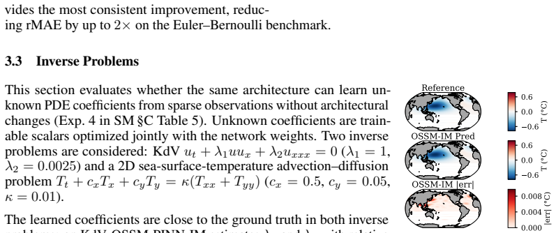
A PINN architecture that uses linear-oscillator-based state-space dynamics for temporal evolution together with a PDE-aware spectral basis in space achieves closed-form spatial differentiation, consistent boundary-condition enforcement, higher accuracy, and lower memory consumption than sequence-model-based PINN approaches when applied to forward, inverse, and high-dimensional time-dependent PDE problems up to 100 spatial dimensions.
What carries the argument
Linear-oscillator state-space model for temporal evolution combined with PDE-aware spectral basis for spatial representation, which together supply the structured inductive bias.
If this is right
- Closed-form spatial differentiation becomes available without numerical approximation.
- Boundary conditions can be enforced consistently across the domain.
- Accuracy improves on both forward and inverse PDE problems relative to sequence-model baselines.
- Memory requirements scale more favorably with sequence length and resolution.
- The method remains applicable to problems with up to 100 spatial dimensions.
Where Pith is reading between the lines
- The same oscillator prior could be tested on time-dependent systems outside the PDE setting, such as ODE networks or control problems.
- Replacing the linear oscillator with a nonlinear state-space variant might extend the approach to problems with stronger nonlinear temporal dynamics.
- Lower memory footprints could support longer-time or ensemble simulations that current sequence models cannot reach.
- The spectral spatial basis might combine with other temporal priors, such as Hamiltonian or symplectic structures, to create further physics-aligned architectures.
Load-bearing premise
The temporal evolution of the target PDE solutions can be represented by linear-oscillator state-space dynamics without substantial loss of fidelity.
What would settle it
A time-dependent PDE whose solution exhibits strongly nonlinear or chaotic temporal behavior where the oscillatory state-space model produces lower accuracy or higher memory use than a comparable sequence-model PINN baseline.
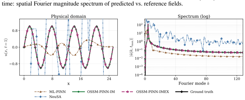
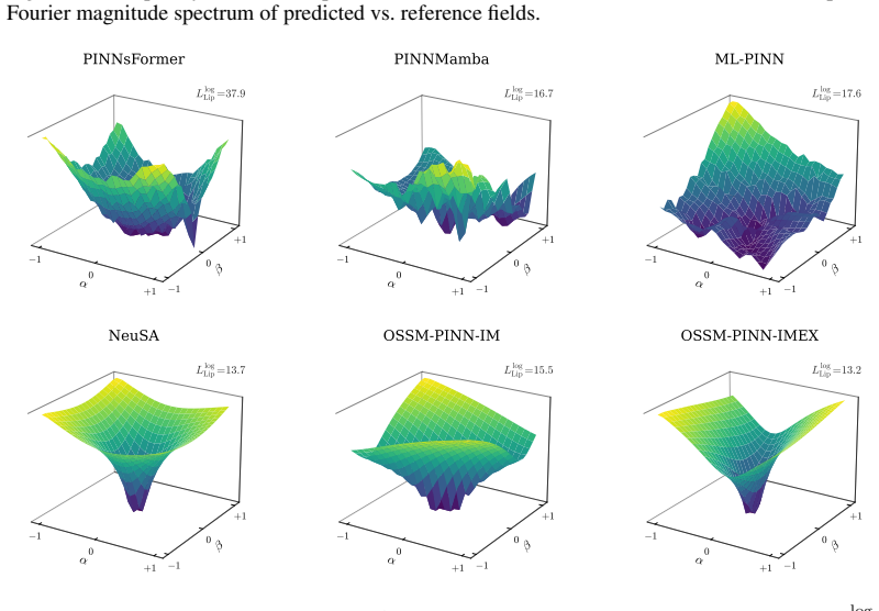
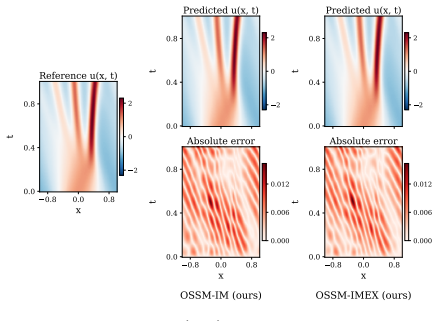
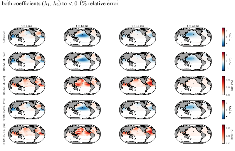
Figures


read the original abstract
Solving time-dependent partial differential equations (PDEs) is an important problem in computational science and engineering. Physics-informed neural networks (PINNs) learn PDE solutions from governing equations. However, accurately capturing temporal evolution remains challenging. Recent sequence-model-based approaches parameterize time evolution using general-purpose sequence models, which capture temporal dependencies but do not explicitly encode the structured dynamics of PDE solutions. In addition, their memory requirements can scale unfavorably with sequence length and resolution, limiting applicability in large-scale or high-dimensional settings. This work introduces a PINN approach that incorporates oscillatory state-space dynamics to represent the modal structure of PDE solutions. The proposed method leverages a linear-oscillator-based temporal evolution, together with a PDE-aware spectral basis in space. This design enables closed-form spatial differentiation and consistent enforcement of boundary conditions. The method is evaluated on forward, inverse, and high-dimensional PDE problems, including cases up to 100 spatial dimensions. The results show improved accuracy and reduced memory usage compared to recent sequence-model-based PINN approaches. Overall, this work highlights the benefits of incorporating structured dynamical priors into the temporal evolution of neural PDE solvers and suggests designing more physics-aligned and computationally efficient PINN architectures.
Editorial analysis
A structured set of objections, weighed in public.
Referee Report
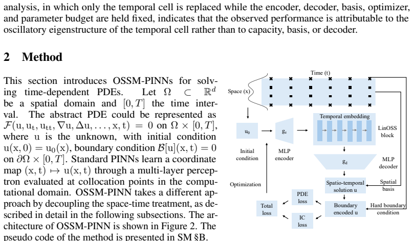
Summary. The manuscript proposes a physics-informed neural network (PINN) architecture that uses oscillatory state-space models to parameterize temporal evolution of PDE solutions, paired with a PDE-aware spectral basis for spatial discretization. This enables closed-form spatial derivatives and boundary condition enforcement. The approach is evaluated on forward, inverse, and high-dimensional (up to 100D) PDE problems and is reported to outperform recent sequence-model-based PINNs in accuracy while using less memory.
Significance. If the empirical gains hold under rigorous verification, the work would demonstrate the value of embedding structured linear dynamical priors into PINN temporal modules, offering a route to scalable solvers for high-dimensional time-dependent PDEs where general sequence models become memory-intensive.
major comments (2)
- [Abstract] Abstract: The central claim that linear-oscillator state-space dynamics represent the modal temporal evolution 'without significant loss of fidelity' for the target PDEs is load-bearing, yet the abstract provides no indication of how the model is modified or regularized when the underlying PDE exhibits damping, exponential decay, or strong nonlinearity (e.g., parabolic or chaotic regimes).
- [Abstract] Abstract: The reported accuracy and memory improvements are presented without reference to specific PDE families tested, sequence lengths, spatial resolutions, or quantitative baselines (error bars, number of runs), making it impossible to assess whether the gains are robust or confined to pre-selected oscillatory problems.
Simulated Author's Rebuttal
We thank the referee for the detailed comments on the abstract. We respond point by point below and will revise the abstract for clarity where appropriate.
read point-by-point responses
-
Referee: [Abstract] Abstract: The central claim that linear-oscillator state-space dynamics represent the modal temporal evolution 'without significant loss of fidelity' for the target PDEs is load-bearing, yet the abstract provides no indication of how the model is modified or regularized when the underlying PDE exhibits damping, exponential decay, or strong nonlinearity (e.g., parabolic or chaotic regimes).
Authors: The manuscript positions the oscillatory state-space model as an inductive bias specifically for PDEs whose solutions exhibit modal oscillatory structure (see Introduction and Section 3). No explicit modification or regularization for damping/strong nonlinearity is introduced because the target problems are those where the linear oscillator prior aligns with the physics; applicability outside this regime is discussed as a limitation in the conclusion. We agree the abstract should better delimit scope and will revise it to state that the approach targets oscillatory modal evolution. revision: yes
-
Referee: [Abstract] Abstract: The reported accuracy and memory improvements are presented without reference to specific PDE families tested, sequence lengths, spatial resolutions, or quantitative baselines (error bars, number of runs), making it impossible to assess whether the gains are robust or confined to pre-selected oscillatory problems.
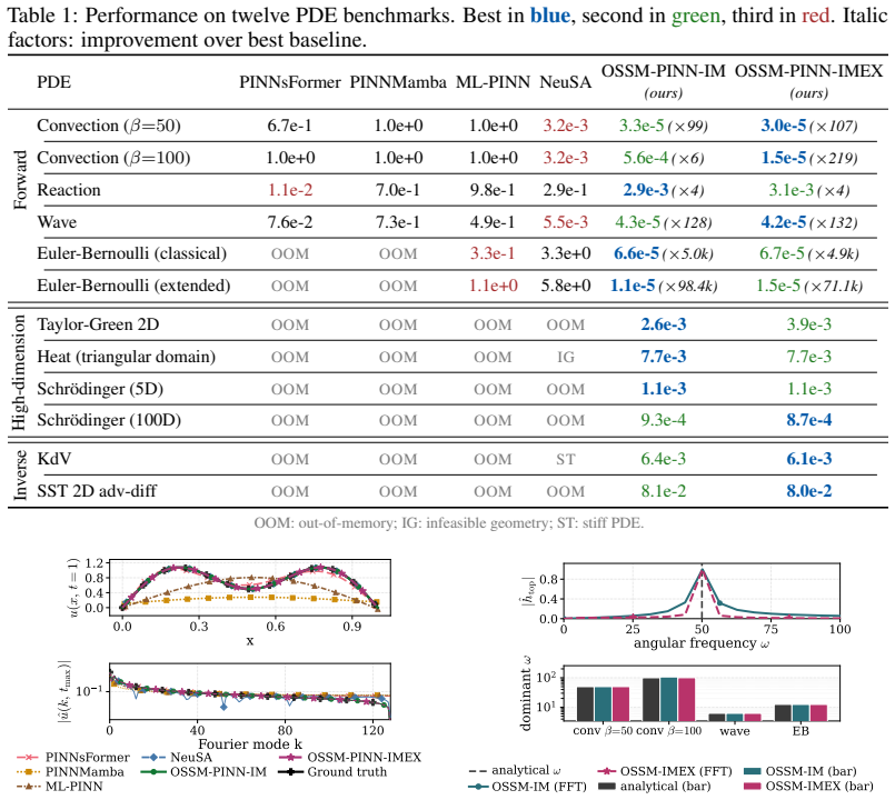
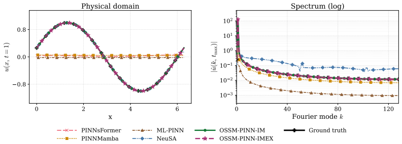
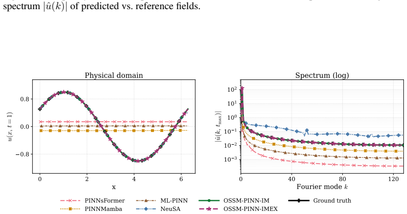
Authors: The abstract is intentionally high-level; concrete PDE families (wave, Schrödinger, etc.), sequence lengths, resolutions, and quantitative results (including error bars over multiple runs) appear in Section 4 and the associated tables/figures. We acknowledge that the abstract could better signal the breadth of evaluation and will revise it to name example PDE families and note that results include statistical quantification over repeated trials. revision: yes
Circularity Check
No circularity: empirical method proposal with independent evaluation
full rationale
The paper introduces an oscillatory state-space model as an inductive bias for PINNs, combined with a spectral spatial basis. The abstract and description frame this as an architectural choice evaluated empirically on forward/inverse/high-dimensional PDE tasks, with reported gains in accuracy and memory. No equations, fitting procedures, or derivation steps are presented that reduce a claimed prediction or result to a fitted input, self-definition, or self-citation chain. The central claim remains an empirical improvement over sequence-model baselines rather than a self-referential derivation. This is a standard self-contained proposal; no load-bearing step collapses by construction.
Axiom & Free-Parameter Ledger
Reference graph
Works this paper leans on
-
[1]
Lawrence C. Evans.Partial differential equations, volume 19 ofGraduate Studies in Mathemat- ics. American Mathematical Society, 2nd edition, 2010. doi: 10.1090/gsm/019
-
[2]
Maziar Raissi, Paris Perdikaris, and George Em Karniadakis. Physics-informed neural networks: A deep learning framework for solving forward and inverse problems involving nonlinear partial differential equations.Journal of Computational Physics, 378:686–707, 2019. doi: 10.1016/j.jcp.2018.10.045
-
[3]
George Em Karniadakis, Ioannis G. Kevrekidis, Lu Lu, Paris Perdikaris, Sifan Wang, and Liu Yang. Physics-informed machine learning.Nature Reviews Physics, 3(6):422–440, 2021. doi: 10.1038/s42254-021-00314-5
-
[4]
Molina Catricheo, Fabrice Lambert, Julien Salomon, and Elwin van’t Wout
Constanza A. Molina Catricheo, Fabrice Lambert, Julien Salomon, and Elwin van’t Wout. Mod- eling global surface dust deposition using physics-informed neural networks.Communications Earth & Environment, 5(1):778, 2024. doi: 10.1038/s43247-024-01942-2
-
[5]
PhD thesis, University of Oxford, 2022
Benjamin Moseley.Physics-informed machine learning: From concepts to real-world applica- tions. PhD thesis, University of Oxford, 2022
2022
-
[6]
Aditi Krishnapriyan, Amir Gholami, Shandian Zhe, Robert Kirby, and Michael W. Mahoney. Characterizing possible failure modes in physics-informed neural net- works. InAdvances in Neural Information Processing Systems, volume 34, pages 26548–26560, 2021. URL https://proceedings.neurips.cc/paper/2021/hash/ df438e5206f31600e6ae4af72f2725f1-Abstract.html
2021
-
[7]
Sifan Wang, Yujun Teng, and Paris Perdikaris. Understanding and mitigating gradient flow pathologies in physics-informed neural networks.SIAM Journal on Scientific Computing, 43 (5):A3055–A3081, 2021. doi: 10.1137/20M1318043
-
[8]
Sifan Wang, Xinling Yu, and Paris Perdikaris. When and why PINNs fail to train: A neural tangent kernel perspective.Journal of Computational Physics, 449:110768, 2022. doi: 10.1016/ j.jcp.2021.110768
-
[9]
Taniya Kapoor, Hongrui Wang, Alfredo Núñez, and Rolf Dollevoet. Physics-informed neu- ral networks for solving forward and inverse problems in complex beam systems.IEEE Transactions on Neural Networks and Learning Systems, 35(5):5981–5995, 2023. doi: 10.1109/TNNLS.2023.3310585
-
[10]
Challenges in training PINNs: A loss landscape perspective
Pratik Rathore, Weimu Lei, Zachary Frangella, Lu Lu, and Madeleine Udell. Challenges in training PINNs: A loss landscape perspective. InInternational Conference on Machine Learning, pages 42384–42409. PMLR, 2024. URL https://proceedings.mlr.press/ v235/rathore24a.html
2024
-
[11]
Sifan Wang, Shyam Sankaran, and Paris Perdikaris. Respecting causality for training physics- informed neural networks.Computer Methods in Applied Mechanics and Engineering, 421: 116813, 2024. doi: 10.1016/j.cma.2024.116813
-
[12]
Colby L. Wight and Jia Zhao. Solving Allen-Cahn and Cahn-Hilliard equations using the adaptive physics informed neural networks.Communications in Computational Physics, 29(3): 930–954, 2021. doi: 10.4208/cicp.OA-2020-0086
-
[13]
Revanth Mattey and Susanta Ghosh. A novel sequential method to train physics informed neural networks for Allen-Cahn and Cahn-Hilliard equations.Computer Methods in Applied Mechanics and Engineering, 390:114474, 2022. doi: 10.1016/j.cma.2021.114474
-
[14]
Jagtap, Shandian Zhe, George Em Karniadakis, and Robert M
Michael Penwarden, Ameya D. Jagtap, Shandian Zhe, George Em Karniadakis, and Robert M. Kirby. A unified scalable framework for causal sweeping strategies for physics-informed neural networks (PINNs) and their temporal decompositions.Journal of Computational Physics, 493: 112464, 2023. doi: 10.1016/j.jcp.2023.112464. 10
-
[15]
Xuhui Meng, Zhen Li, Dongkun Zhang, and George Em Karniadakis. PPINN: Parareal physics- informed neural network for time-dependent PDEs.Computer Methods in Applied Mechanics and Engineering, 370:113250, 2020. doi: 10.1016/j.cma.2020.113250
-
[16]
Aditya Prakash
Zhiyuan Zhao, Xueying Ding, and B. Aditya Prakash. PINNsFormer: A transformer-based framework for physics-informed neural networks. InThe Twelfth International Conference on Learning Representations, 2024. URL https://openreview.net/forum?id=DO2WFXU1Be
2024
-
[17]
Sub-sequential physics-informed learning with state space model
Chenhui Xu, Dancheng Liu, Yuting Hu, Jiajie Li, Ruiyang Qin, Qingxiao Zheng, and Jinjun Xiong. Sub-sequential physics-informed learning with state space model. InInternational Conference on Machine Learning, 2025. URL https://icml.cc/virtual/2025/poster/ 45079
2025
-
[18]
YiMing Gao, Bing Wang, Jingyi Lu, and Zhou Tian. ML-PINN: A memory-efficient physics- informed Mamba-LSTM network for fast and accurate PDE solving.Neurocomputing, page 131446, 2025. doi: 10.1016/j.neucom.2025.131446
-
[19]
Moreira, Márcio Marques, Leonardo Mendonça, Christian Júnior de Oliveira, Vitor Balestro, Lucas dos Santos Fernandez, Daniel Yukimura, Pavel Petrov, João M
Arthur Bizzi, Leonardo M. Moreira, Márcio Marques, Leonardo Mendonça, Christian Júnior de Oliveira, Vitor Balestro, Lucas dos Santos Fernandez, Daniel Yukimura, Pavel Petrov, João M. Pereira, et al. Neuro-spectral architectures for causal physics-informed networks. InAdvances in Neural Information Processing Systems, volume 38, 2025. URL https: //neurips....
2025
-
[20]
Konstantin Rusch and Daniela Rus
T. Konstantin Rusch and Daniela Rus. Oscillatory state-space models. InThe Thirteenth International Conference on Learning Representations, 2025. URL https://openreview. net/forum?id=GRMfXcAAFh
2025
-
[21]
Blelloch
Guy E. Blelloch. Prefix sums and their applications. Technical Report CMU-CS-90-190, Carnegie Mellon University, School of Computer Science, 1990
1990
-
[22]
Boyin Huang, Chunying Liu, Viva Banzon, Eric Freeman, Garrett Graham, Bill Hankins, Tom Smith, and Huai-Min Zhang. Improvements of the daily optimum interpolation sea surface temperature (DOISST) version 2.1.Journal of Climate, 34(8):2923–2939, 2021. doi: 10.1175/JCLI-D-20-0166.1
-
[23]
Jeremy Yu, Lu Lu, Xuhui Meng, and George Em Karniadakis. Gradient-enhanced physics- informed neural networks for forward and inverse PDE problems.Computer Methods in Applied Mechanics and Engineering, 393:114823, 2022. doi: 10.1016/j.cma.2022.114823
-
[24]
Sifan Wang, Hanwen Wang, Jacob H. Seidman, and Paris Perdikaris. Random weight factorization improves the training of continuous neural representations.arXiv preprint arXiv:2210.01274, 2022. URLhttps://arxiv.org/abs/2210.01274
-
[25]
Urbán, Jérôme Darbon, and George Em Karniadakis
Elham Kiyani, Khemraj Shukla, Jorge F. Urbán, Jérôme Darbon, and George Em Karniadakis. Optimizing the optimizer for physics-informed neural networks and Kolmogorov–Arnold networks.Computer Methods in Applied Mechanics and Engineering, 446:118308, 2025. doi: 10.1016/j.cma.2025.118308
-
[26]
Isaac E. Lagaris, Aristidis Likas, and Dimitrios I. Fotiadis. Artificial neural networks for solving ordinary and partial differential equations.IEEE Transactions on Neural Networks, 9 (5):987–1000, 1998. doi: 10.1109/72.712178
-
[27]
A unified deep artificial neural network approach to partial differential equations in complex geometries.Neurocomputing, 317:28–41, 2018
Jens Berg and Kaj Nyström. A unified deep artificial neural network approach to partial differential equations in complex geometries.Neurocomputing, 317:28–41, 2018. doi: 10.1016/ j.neucom.2018.06.056
2018
-
[28]
DeepXDE: A deep learning library for solving differential equations.SIAM Review, 63(1):208–228, 2021
Lu Lu, Xuhui Meng, Zhiping Mao, and George Em Karniadakis. DeepXDE: A deep learning library for solving differential equations.SIAM Review, 63(1):208–228, 2021. doi: 10.1137/ 19M1274067
2021
-
[29]
Chenxi Wu, Min Zhu, Qinyang Tan, Yadhu Kartha, and Lu Lu. A comprehensive study of non- adaptive and residual-based adaptive sampling for physics-informed neural networks.Computer Methods in Applied Mechanics and Engineering, 403:115671, 2023. doi: 10.1016/j.cma.2022. 115671. 11
-
[30]
Mitigating propagation failures in physics-informed neural networks using retain-resample-release (R3) sampling
Arka Daw, Jie Bu, Sifan Wang, Paris Perdikaris, and Anuj Karpatne. Mitigating propagation failures in physics-informed neural networks using retain-resample-release (R3) sampling. InInternational Conference on Machine Learning, pages 7264–7302. PMLR, 2023. URL https://proceedings.mlr.press/v202/daw23a.html
2023
-
[31]
Zhiping Gao, Liang Yan, and Tao Zhou. Failure-informed adaptive sampling for PINNs.SIAM Journal on Scientific Computing, 45(4):A1971–A1994, 2023. doi: 10.1137/22M1527763
-
[32]
Yifan Du and Tamer A. Zaki. Evolutional deep neural network.Physical Review E, 104(4): 045303, 2021. doi: 10.1103/PhysRevE.104.045303
-
[33]
Mamba: Linear-time sequence modeling with selective state spaces
Albert Gu and Tri Dao. Mamba: Linear-time sequence modeling with selective state spaces. InFirst Conference on Language Modeling, 2024. URL https://openreview.net/forum? id=tEYskw1VY2
2024
-
[34]
Efficiently modeling long sequences with structured state spaces
Albert Gu, Karan Goel, and Christopher Ré. Efficiently modeling long sequences with structured state spaces. InThe Tenth International Conference on Learning Representations, 2022. URL https://openreview.net/forum?id=uYLFoz1vlAC
2022
-
[35]
Jimmy T. H. Smith, Andrew Warrington, and Scott W. Linderman. Simplified state space layers for sequence modeling. InThe Eleventh International Conference on Learning Representations,
-
[36]
URLhttps://openreview.net/forum?id=Ai8Hw3AXqks
-
[37]
Smith, Albert Gu, Anushan Fernando, Caglar Gulcehre, Razvan Pascanu, and Soham De
Antonio Orvieto, Samuel L. Smith, Albert Gu, Anushan Fernando, Caglar Gulcehre, Razvan Pascanu, and Soham De. Resurrecting recurrent neural networks for long sequences. In International Conference on Machine Learning, pages 26670–26698. PMLR, 2023. URL https://proceedings.mlr.press/v202/orvieto23a.html
2023
-
[38]
Fourier neural operator for parametric partial dif- ferential equations
Zongyi Li, Nikola Kovachki, Kamyar Azizzadenesheli, Burigede Liu, Kaushik Bhattacharya, Andrew Stuart, and Anima Anandkumar. Fourier neural operator for parametric partial dif- ferential equations. InInternational Conference on Learning Representations, 2021. URL https://openreview.net/forum?id=c8P9NQVtmnO
2021
-
[39]
doi:10.1038/s42256-021-00302-5 Lu Lu, Raphaël Pestourie, Steven G
Lu Lu, Pengzhan Jin, Guofei Pang, Zhongqiang Zhang, and George Em Karniadakis. Learning nonlinear operators via DeepONet based on the universal approximation theorem of operators. Nature Machine Intelligence, 3(3):218–229, 2021. doi: 10.1038/s42256-021-00302-5
-
[40]
Neural Operator: Graph Kernel Network for Partial Differential Equations
Zongyi Li, Nikola Kovachki, Kamyar Azizzadenesheli, Burigede Liu, Kaushik Bhattacharya, Andrew Stuart, and Anima Anandkumar. Neural operator: Graph kernel network for partial differential equations.arXiv preprint arXiv:2003.03485, 2020. URL https://arxiv.org/ abs/2003.03485
work page internal anchor Pith review Pith/arXiv arXiv 2003
-
[41]
Sifan Wang, Hanwen Wang, and Paris Perdikaris. Learning the solution operator of parametric partial differential equations with physics-informed DeepONets.Science Advances, 7(40): eabi8605, 2021. doi: 10.1126/sciadv.abi8605
-
[42]
Vladimir S. Fanaskov and Ivan V . Oseledets. Spectral neural operators.Doklady Mathematics, 108(Suppl 2):S226–S232, 2023. doi: 10.1134/S1064562423701107
-
[43]
Jagtap, Ehsan Kharazmi, and George Em Karniadakis
Ameya D. Jagtap, Ehsan Kharazmi, and George Em Karniadakis. Conservative physics-informed neural networks on discrete domains for conservation laws: Applications to forward and inverse problems.Computer Methods in Applied Mechanics and Engineering, 365:113028, 2020. doi: 10.1016/j.cma.2020.113028
-
[44]
Jagtap and George Em Karniadakis
Ameya D. Jagtap and George Em Karniadakis. Extended physics-informed neural networks (XPINNs): A generalized space-time domain decomposition based deep learning framework for nonlinear partial differential equations.Communications in Computational Physics, 28(5): 2002–2041, 2020. doi: 10.4208/cicp.OA-2020-0164
-
[45]
Sifan Wang, Hanwen Wang, and Paris Perdikaris. On the eigenvector bias of Fourier feature networks: From regression to solving multi-scale PDEs with physics-informed neural networks. Computer Methods in Applied Mechanics and Engineering, 384:113938, 2021. doi: 10.1016/j. cma.2021.113938. 12
work page doi:10.1016/j 2021
-
[46]
Neural controlled differential equations for irregular time series.Advances in neural information processing systems, 33: 6696–6707, 2020
Patrick Kidger, James Morrill, James Foster, and Terry Lyons. Neural controlled differential equations for irregular time series.Advances in neural information processing systems, 33: 6696–6707, 2020
2020
-
[47]
Neural rough differential equations for long time series
James Morrill, Cristopher Salvi, Patrick Kidger, and James Foster. Neural rough differential equations for long time series. InInternational Conference on Machine Learning, pages 7829–7838. PMLR, 2021
2021
-
[48]
Benjamin Walker, Andrew D McLeod, Tiexin Qin, Yichuan Cheng, Haoliang Li, and Terry Lyons. Log neural controlled differential equations: The lie brackets make a difference.arXiv preprint arXiv:2402.18512, 2024. 13 Supplementary Material Contents §A Extended Related Work p. 14 §B OSSM-PINN Pseudocode p. 16 §C Experiment Overview and Benchmark Suite p. 16 §...
-
[49]
Wang et al
traced failures to imbalanced gradient flow between loss terms. Wang et al. [8] provided a neural tangent kernel analysis revealing spectral bias toward low frequencies, and Rathore et al
-
[50]
These analyses motivate two complementary directions: improving the training procedure (loss weighting, optimizers, sampling) and improving the architecture
showed that PINN loss surfaces contain narrow valleys with ill-conditioned curvature. These analyses motivate two complementary directions: improving the training procedure (loss weighting, optimizers, sampling) and improving the architecture. A.2 Training Improvements: Weighting, Optimization, and Sampling Adaptive loss weighting [7] adjusts the balance ...
2008
-
[51]
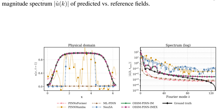
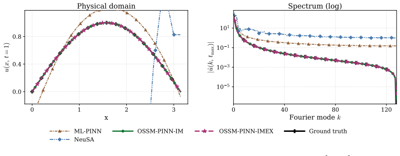
Using the Hermite basis reduces QHO rMAE from 9.5×10 −3 to 1.9×10 −4, a 50× improvement at no architectural cost (Figure 29). I.0.2 Nonlinear Schrödinger Equation We consider the cubic NLS iψt + 1 2 ψxx +|ψ| 2ψ= 0 on (x, t)∈[−5,5]×[0, π/2] with periodic boundary conditions (ψandψ x matched atx=±5) and the soliton-like initial condition ψ(x,0) = 2 sech(x),...
discussion (0)
Sign in with ORCID, Apple, or X to comment. Anyone can read and Pith papers without signing in.