A Temporal Spatial Minimax Rate for Smoothly-Varying Distributions in Wasserstein Space
Pith reviewed 2026-06-27 20:29 UTC · model grok-4.3
The pith
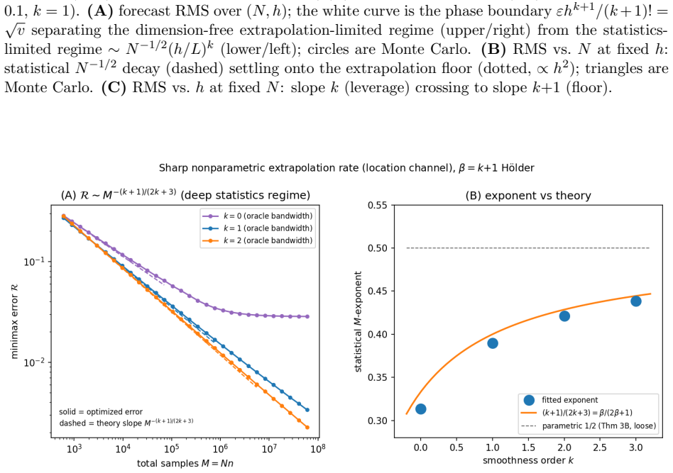
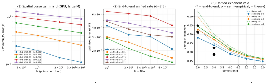
The minimax risk for estimating a future distribution along a Wasserstein curve under velocity smoothness k scales as M to the exponent γ_d(k+1)/(k+1+γ_d) with γ_d = min(1/d, 1/2).
A machine-rendered reading of the paper's core claim, the machinery that carries it, and where it could break.
Core claim
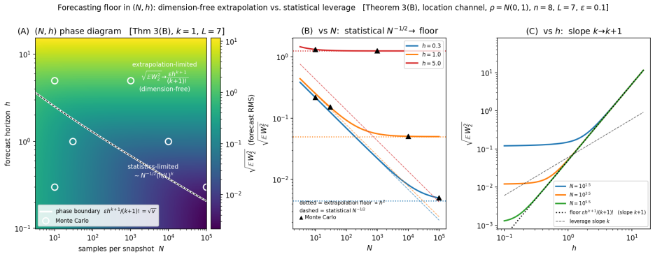
Over regular, locally transport-rich subclasses satisfying the adiabatic bound ||∇_t^k v|| ≤ ε on the k-th covariant derivative of the velocity field, every estimator of μ_{t_n + h} incurs W_2-risk with M-exponent γ_d(k+1)/(k+1 + γ_d), γ_d = min(1/d, 1/2). This follows from a temporal-to-spatial reduction in which the smoothness budget defines a reachable W_2-ball into which a transport packing is embedded along the time axis; the information of the entire snapshot experiment is then controlled by a Fano argument.
What carries the argument
The temporal-to-spatial reduction that embeds a classical spatial transport packing into the reachable W_2-ball defined by the adiabatic smoothness budget along the time axis, thereby controlling the full-window experiment via a Fano argument.
If this is right
- The bound recovers the static distribution estimation rate M^{-γ_d} as k tends to infinity.
- For k = 0 the lower bound is of order M^{-1/(d+1)} when d ≥ 3.
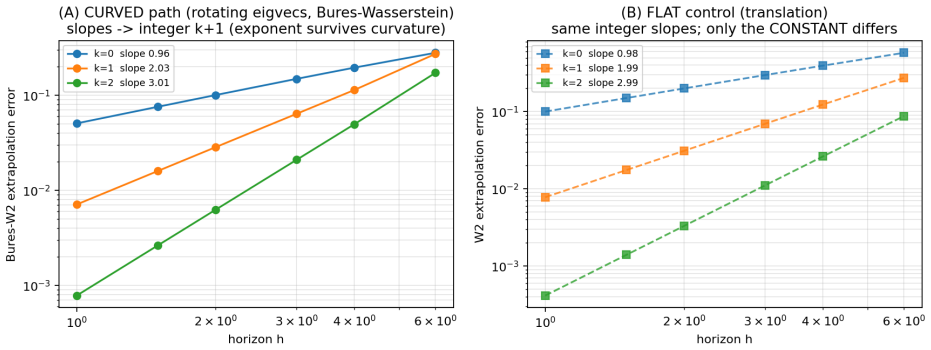
- An irreducible extrapolation cost of order ε h^{k+1} remains even when the entire past is known exactly.
- The lower bound holds in design-weighted form for arbitrary observation times and simplifies to the stated closed-form exponent in the equispaced regime.
Where Pith is reading between the lines
- A matching upper bound for general k remains open outside translation-invariant submodels.
- The reduction technique could be tested on other optimal-transport metrics or on curves evolving in different metric spaces.
- The conditional upper bounds obtained via covariant estimators indicate that separate control of geometry-estimation bias may suffice to close the gap for k ≥ 1.
Load-bearing premise
The distributions belong to regular, locally transport-rich subclasses that satisfy the adiabatic bound on the k-th covariant derivative of the velocity field.
What would settle it
Constructing an estimator whose risk on some sequence of such curve classes decays strictly faster than M to the power γ_d(k+1)/(k+1 + γ_d), or exhibiting a curve class in the stated family for which the embedded packing size cannot be controlled by the given smoothness budget.
Figures


read the original abstract
We study the minimax rate of estimating a future value $\mu_{t_n+h}$ of a curve $t\mapsto\mu_t$ in the $2$-Wasserstein space $\mathcal{P}_2(\mathbb{R}^d)$ from finitely many noisy snapshots of its past, under an adiabatic bound $\|\nabla_t^k v\|\le\varepsilon$ on the $k$-th covariant derivative of the velocity field. Our central result is a unified temporal-spatial minimax lower bound: over regular, locally transport-rich subclasses, every estimator incurs $W_2$-risk with $M$-exponent $\gamma_d(k+1)/(k+1+\gamma_d)$, $\gamma_d=\min(1/d,1/2)$ ($M$ the total sample size). It follows from a temporal-to-spatial reduction: the smoothness budget defines a reachable $W_2$-ball into which a transport packing is embedded along the time axis, and the information of the entire snapshot experiment is controlled by a Fano argument -- the spatial packing is classical, but its smoothness-admissible temporal embedding and the full-window analysis are new. The bound interpolates a dimension-free extrapolation floor of order $\varepsilon h^{k+1}$ -- the irreducible cost of an unobserved future, present even with the exact past -- and the spatial estimation curse $M^{-\gamma_d}$, recovering the static distribution-estimation rate as $k\to\infty$. We state the lower bound in a design-dependent form -- with a design-weighted effective sample size -- valid for arbitrary observation times, and obtain the closed-form exponent in the dense (equispaced) regime. The matching upper bound is established at $k=0$ (rate $M^{-1/(d+1)}$, $d\ge3$) and, in a translation submodel, for all $k$; for $k\ge1$ a covariant estimator attains the rate conditionally on two estimates (a comparison-geometry bias bound and an optimal-transport map-estimation rate), leaving the unconditional general-$k$ upper bound as an open problem. Numerical experiments on synthetic curved and flat families corroborate the predicted exponents.
Editorial analysis
A structured set of objections, weighed in public.
Referee Report
Summary. The paper claims a unified minimax lower bound on the W_2-risk of estimating a future snapshot μ_{t_n+h} of a curve t ↦ μ_t in P_2(R^d), under an adiabatic bound ||∇_t^k v|| ≤ ε on the k-th covariant derivative of the velocity field. The bound has total-sample-size exponent γ_d(k+1)/(k+1+γ_d) with γ_d = min(1/d,1/2), obtained by embedding a classical spatial transport packing into a time-dependent curve that respects the adiabatic constraint and then applying Fano's inequality to the resulting family of snapshot laws. The lower bound interpolates the irreducible extrapolation cost ε h^{k+1} and the static spatial rate M^{-γ_d}; matching upper bounds are proved for k=0 (rate M^{-1/(d+1)} when d≥3) and conditionally for all k in a translation submodel, while the unconditional general-k upper bound remains open. Numerical experiments on synthetic families are reported to corroborate the exponents.
Significance. If the central lower-bound claim holds, the result supplies the first unified temporal-spatial rate for dynamic distribution estimation in Wasserstein space that accounts for both smoothness budget and observation design. The temporal-to-spatial reduction together with the full-window Fano analysis constitute a genuine technical contribution; the design-dependent form of the bound is also useful. The partial upper bounds and the numerical corroboration add value, though the open general-k upper-bound question limits immediate applicability.
major comments (2)
- [temporal-to-spatial reduction (central result)] The lower-bound argument requires that the adiabatically embedded packing remain inside the 'regular, locally transport-rich' subclass so that the spatial packing still yields the claimed KL separation. The manuscript does not supply an explicit verification that, for the chosen packing radius and admissible ε, the induced velocity field keeps optimal maps sufficiently non-degenerate and prevents support collapse. This verification is load-bearing for the Fano step and therefore for the stated exponent.
- [upper-bound statements] The matching upper bound is proved unconditionally only for k=0 and, for k≥1, only conditionally on two auxiliary estimates (comparison-geometry bias bound and OT-map rate) inside a translation submodel. Because the paper's main claim is the lower bound, this gap does not invalidate the central result, but it does affect the strength of the 'unified rate' narrative.
minor comments (2)
- [preliminaries] Notation for the covariant derivative ∇_t^k v and the precise definition of the 'locally transport-rich' subclass should be collected in a single preliminary section rather than introduced piecemeal.
- [main theorem] The design-weighted effective sample size is introduced in the lower-bound statement; a short remark clarifying how the dense equispaced regime recovers the closed-form exponent would improve readability.
Simulated Author's Rebuttal
We thank the referee for the thoughtful review and for recognizing the technical contribution of the temporal-to-spatial reduction and the Fano analysis. We address each major comment below.
read point-by-point responses
-
Referee: [temporal-to-spatial reduction (central result)] The lower-bound argument requires that the adiabatically embedded packing remain inside the 'regular, locally transport-rich' subclass so that the spatial packing still yields the claimed KL separation. The manuscript does not supply an explicit verification that, for the chosen packing radius and admissible ε, the induced velocity field keeps optimal maps sufficiently non-degenerate and prevents support collapse. This verification is load-bearing for the Fano step and therefore for the stated exponent.
Authors: We agree that the manuscript would benefit from an explicit verification to ensure the construction remains within the specified subclass. In the revised version, we will add a detailed check in the proof of the lower bound, showing that the chosen packing radius and ε ensure the velocity fields induce optimal maps that are sufficiently non-degenerate (e.g., with Jacobians bounded away from zero) and that supports do not collapse, thereby preserving the KL separation required for Fano's inequality. revision: yes
-
Referee: [upper-bound statements] The matching upper bound is proved unconditionally only for k=0 and, for k≥1, only conditionally on two auxiliary estimates (comparison-geometry bias bound and OT-map rate) inside a translation submodel. Because the paper's main claim is the lower bound, this gap does not invalidate the central result, but it does affect the strength of the 'unified rate' narrative.
Authors: We acknowledge the limitation in the upper bounds as described. The central claim is indeed the lower bound, which provides the unified rate. We will revise the abstract, introduction, and conclusion to more clearly state that the matching upper bound is available unconditionally only for k=0 and conditionally in a submodel for higher k, and to explicitly note the open problem for the general case. This will ensure the narrative accurately reflects the scope of the results. revision: yes
Circularity Check
No circularity in derivation chain
full rationale
The central lower bound is obtained by embedding a classical spatial transport packing into a time-dependent curve obeying the adiabatic bound, then applying the standard Fano inequality to the resulting family of snapshot laws. The paper explicitly states that the spatial packing is classical while the temporal embedding and full-window analysis are new; no equation reduces the claimed exponent to a fitted parameter, a self-defined quantity, or a load-bearing self-citation. The result is presented as an interpolation between the known dimension-free extrapolation floor and the static estimation rate, with the derivation remaining self-contained against external benchmarks.
Axiom & Free-Parameter Ledger
axioms (2)
- standard math Fano inequality applies to the constructed temporal-spatial packing
- domain assumption Wasserstein geometry admits transport maps and covariant derivatives of velocity fields
Reference graph
Works this paper leans on
-
[1]
Ambrosio, N
L. Ambrosio, N. Gigli, G. Savar´ e.Gradient Flows in Metric Spaces and in the Space of Probability Measures. 2nd ed., Lectures in Math. ETH Z¨ urich, Birkh¨ auser, 2008
2008
-
[2]
N. Gigli. Second order analysis on (P 2(M), W 2).Mem. Amer. Math. Soc.216 (2012), no. 1018
2012
-
[3]
Villani.Optimal Transport: Old and New
C. Villani.Optimal Transport: Old and New. Grundlehren der math. Wissenschaften 338, Springer, 2009. 10
2009
-
[4]
Second order models for optimal transport and cubic splines on the Wasserstein space
J.-D. Benamou, T. O. Gallou¨ et, F.-X. Vialard. Second-order models for optimal transport and cubic splines on the Wasserstein space.Found. Comput. Math.19 (2019), 1113–1143. doi:10.1007/s10208-019-09425-z; arXiv:1801.04144
work page internal anchor Pith review Pith/arXiv arXiv doi:10.1007/s10208-019-09425-z 2019
- [5]
- [6]
-
[7]
Z. Wang, Y. Araki. Functional time series forecasting of distributions: a Koopman–Wasserstein ap- proach.Behaviormetrika(2025).doi:10.1007/s41237-025-00278-1; arXiv:2507.07570
-
[8]
L. Ghodrati, V. M. Panaretos. Minimax rate for optimal transport regression between distributions. Statist. Probab. Lett.194 (2022), 109758.doi:10.1016/j.spl.2022.109758; arXiv:2206.01447
-
[9]
Fournier, A
N. Fournier, A. Guillin. On the rate of convergence in Wasserstein distance of the empirical measure. Probab. Theory Related Fields162 (2015), 707–738
2015
-
[10]
Niles-Weed, Q
J. Niles-Weed, Q. Berthet. Minimax estimation of smooth densities in Wasserstein distance.Ann. Statist.50 (2022), no. 3, 1519–1540
2022
- [11]
-
[12]
C. J. Stone. Optimal rates of convergence for nonparametric estimators.Ann. Statist.8 (1980), no. 6, 1348–1360
1980
-
[13]
A. B. Tsybakov.Introduction to Nonparametric Estimation. Springer Ser. in Statist., Springer, 2009
2009
-
[14]
F. Otto. The geometry of dissipative evolution equations: the porous medium equation.Comm. Partial Differential Equations26 (2001), no. 1–2, 101–174
2001
-
[15]
Benamou, Y
J.-D. Benamou, Y. Brenier. A computational fluid mechanics solution to the Monge–Kantorovich mass transfer problem.Numer. Math.84 (2000), no. 3, 375–393
2000
-
[16]
J. Weed, F. Bach. Sharp asymptotic and finite-sample rates of convergence of empirical measures in Wasserstein distance.Bernoulli25 (2019), no. 4A, 2620–2648
2019
-
[17]
R. M. Dudley. The speed of mean Glivenko–Cantelli convergence.Ann. Math. Statist.40 (1969), no. 1, 40–50
1969
-
[18]
Schiebinger, J
G. Schiebinger, J. Shu, M. Tabaka, et al. Optimal-transport analysis of single-cell gene expression identifies developmental trajectories in reprogramming.Cell176 (2019), no. 4, 928–943
2019
-
[19]
H. Lavenant, S. Zhang, Y.-H. Kim, G. Schiebinger. Toward a mathematical theory of trajectory infer- ence.Ann. Appl. Probab.34 (2024), no. 1A, 428–500.doi:10.1214/23-AAP1969; arXiv:2102.09204
-
[20]
Dahlhaus
R. Dahlhaus. Fitting time series models to nonstationary processes.Ann. Statist.25 (1997), no. 1, 1–37
1997
-
[21]
J. Gama, I. ˇZliobait˙ e, A. Bifet, M. Pechenizkiy, A. Bouchachia. A survey on concept drift adaptation. ACM Comput. Surv.46 (2014), no. 4, art. 44
2014
-
[22]
J. Fan, I. Gijbels.Local Polynomial Modelling and Its Applications. Monographs on Statist. and Appl. Probab. 66, Chapman & Hall, 1996
1996
-
[23]
J.-C. H¨ utter, P. Rigollet. Minimax estimation of smooth optimal transport maps.Ann. Statist.49 (2021), no. 2, 1166–1194. arXiv:1905.05828
arXiv 2021
-
[24]
Plugin estimation of smooth optimal transport maps
T. Manole, S. Balakrishnan, J. Niles-Weed, L. Wasserman. Plugin estimation of smooth optimal trans- port maps.Ann. Statist.52 (2024), no. 3, 966–998.doi:10.1214/24-AOS2379; arXiv:2107.12364. 11
-
[25]
A.-A. Pooladian, J. Niles-Weed. Entropic estimation of optimal transport maps. arXiv:2109.12004, 2021
arXiv 2021
-
[26]
P. T. Fletcher. Geodesic regression and the theory of least squares on Riemannian manifolds.Int. J. Comput. Vis.105 (2013), no. 2, 171–185
2013
-
[27]
M. Cuturi. Sinkhorn distances: lightspeed computation of optimal transport.Adv. Neural Inf. Process. Syst.26 (NIPS 2013), 2292–2300
2013
-
[28]
J. Feydy, T. S´ ejourn´ e, F.-X. Vialard, S.-i. Amari, A. Trouv´ e, G. Peyr´ e. Interpolating between opti- mal transport and MMD using Sinkhorn divergences.Proc. AISTATS, PMLR 89 (2019), 2681–2690. arXiv:1810.08278
Pith/arXiv arXiv 2019
-
[29]
Peyr´ e, M
G. Peyr´ e, M. Cuturi. Computational optimal transport.Found. Trends Mach. Learn.11 (2019), no. 5–6, 355–607
2019
-
[30]
A PDE approach to a 2-dimensional matching problem
L. Ambrosio, F. Stra, D. Trevisan. A PDE approach to a 2-dimensional matching problem.Probab. Theory Related Fields173 (2019), 433–477.doi:10.1007/s00440-018-0837-x; arXiv:1611.04960
work page internal anchor Pith review Pith/arXiv arXiv doi:10.1007/s00440-018-0837-x 2019
-
[31]
R. Peyr´ e. Comparison betweenW 2 distance and ˙H −1 norm, and localization of Wasserstein dis- tance.ESAIM Control Optim. Calc. Var.24 (2018), no. 4, 1489–1501.doi:10.1051/cocv/2017050; arXiv:1104.4631. A Proofs This appendix collects the proofs of the results stated in the main text, in order of appearance. Proof of Lemma 1.(τ x, τy)#ρhas cost|x−y| 2, s...
discussion (0)
Sign in with ORCID, Apple, or X to comment. Anyone can read and Pith papers without signing in.