Minimax Optimal Variance-Aware Regret Bounds for Multinomial Logistic MDPs

Alessandro Rudi (PSL; DI-ENS; INRIA); Pierre Boudart (SIERRA); Pierre Gaillard (Thoth)

arxiv: 2605.19768 · v1 · pith:7WVGP27Knew · submitted 2026-05-19 · 💻 cs.AI · cs.LG· math.ST· stat.ML· stat.TH

Minimax Optimal Variance-Aware Regret Bounds for Multinomial Logistic MDPs

Pierre Boudart (SIERRA) , Pierre Gaillard (Thoth) , Alessandro Rudi (PSL , DI-ENS , Inria) This is my paper

Pith reviewed 2026-05-20 04:52 UTC · model grok-4.3

classification 💻 cs.AI cs.LGmath.STstat.MLstat.TH

keywords reinforcement learningregret boundsmultinomial logistic modelMarkov decision processesvariance-aware analysisminimax optimality

0 comments

The pith

Multinomial logistic MDPs admit a variance-aware regret of order d H squared times average variance times square root T, with a matching lower bound.

A machine-rendered reading of the paper's core claim, the machinery that carries it, and where it could break.

The paper examines episodic MDPs whose transitions follow a multinomial logistic model. It defines a problem-dependent quantity that tracks the normalized average variance of the optimal value function along the trajectory taken by the learner. An algorithm is presented whose regret scales with this quantity rather than with the worst-case constant, recovering prior bounds when variance is large but improving them when the MDP has exploitable structure. A matching lower bound is proved, establishing that the regret complexity of this class of MDPs is now fully characterized up to logarithmic factors.

Core claim

The authors introduce the normalized average variance bar sigma_T of the optimal downstream value function along the learner's trajectory and show that an appropriately designed algorithm attains regret tilde O(d H^2 bar sigma_T sqrt(T)). This quantity is at most 1/2 and can be much smaller under structure; for example it equals O(H^{-1}) in KL-constrained robust MDPs, which removes a full factor of H from the horizon dependence. They also prove a matching Omega(d H^2 bar sigma_T sqrt(T)) lower bound, demonstrating minimax optimality up to logs.

What carries the argument

The normalized average variance bar sigma_T of the optimal downstream value function along the learner's trajectory, which scales the leading term in both the upper and lower regret bounds.

If this is right

In KL-constrained robust MDPs the horizon dependence of the regret improves from H^2 to H.
The new bound recovers the existing worst-case guarantee whenever bar sigma_T is bounded away from zero.
The minimax regret complexity of the entire class of MNL mixture MDPs is now characterized up to logs.
Algorithms that ignore variance information are provably suboptimal on structured instances.

Where Pith is reading between the lines

These are editorial extensions of the paper, not claims the author makes directly.

Analogous variance quantities could be defined and exploited for regret adaptation in other parametric MDP families.
In applied settings one could attempt to estimate bar sigma_T from observed trajectories to forecast the realized regret.
The same technique may extend to infinite-horizon or continuous-state problems once a suitable trajectory-averaged variance can be defined.

Load-bearing premise

Transitions must be generated exactly by a multinomial logistic model and the average variance of the optimal value function must be a well-defined, non-circular constant that can be used directly in the analysis.

What would settle it

An explicit construction of an MNL MDP in which any algorithm incurs regret that exceeds the proposed upper bound by more than logarithmic factors, or in which the lower-bound instance fails to force the claimed Omega rate.

Figures

Figures reproduced from arXiv: 2605.19768 by Alessandro Rudi (PSL, DI-ENS, INRIA), Pierre Boudart (SIERRA), Pierre Gaillard (Thoth).

**Figure 2.** Figure 2: Cumulative regret RegT for different episode lengths H as a function of the episode t. We plot the means ±1 standard deviation across 40 seeds [PITH_FULL_IMAGE:figures/full_fig_p028_2.png] view at source ↗

**Figure 3.** Figure 3: Cumulative regret RegT at T = 1000 episodes normalised by H3/2 as a function of the horizon H. We plot the means ±1 standard deviation across 40 seeds. G Auxiliary Result Lemma 8. For any N ≥ 1 and q ∈]0, 1[, we have N − 1 − (1 − q) N X−1 k=0 q k (N − 1 − k) = 1 − q N 1 − q − 1 . 28 [PITH_FULL_IMAGE:figures/full_fig_p028_3.png] view at source ↗

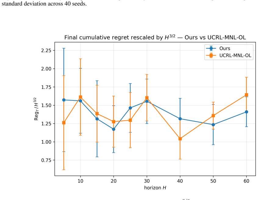
read the original abstract

We study reinforcement learning for episodic Markov Decision Processes (MDPs) whose transitions are modelled by a multinomial logistic (MNL) model. Existing algorithms for MNL mixture MDPs yield a regret of $\smash{\tilde{O}(dH^2\sqrt{T})}$ (Li et al., 2024), where $d$ is the feature dimension, $H$ the episode length, and $T$ the number of episodes. Inspired by the logistic bandit literature (Abeille et al., 2021; Faury et al., 2022; Boudart et al., 2026), we introduce a problem-dependent constant $\bar\sigma\_T \leq 1/2$, measuring the normalised average variance of the optimal downstream value function along the learner's trajectory. We propose an algorithm achieving a regret of $\smash{\tilde{O}(dH^2\bar\sigma\_T\sqrt{T})}$, which recovers the existing bound in the worst case and improves upon it for structured MDPs. For instance, for KL-constrained robust MDPs, $\bar\sigma\_T = O(H^{-1})$, reducing the horizon dependence by a factor $H$. We further establish a matching $\smash{\Omega(dH^2\bar\sigma\_T\sqrt{T})}$ lower bound, proving minimax optimality (up to logarithmic factors) and fully characterising the regret complexity of MNL mixture MDPs for the first time.

Editorial analysis

A structured set of objections, weighed in public.

Desk editor's note, referee report, simulated authors' rebuttal, and a circularity audit. Tearing a paper down is the easy half of reading it; the pith above is the substance, this is the friction.

Desk Editor's Note private letter to a colleague

This paper gives matching upper and lower regret bounds for multinomial logistic MDPs that depend on a trajectory variance term, recovering the prior worst-case rate but improving it in structured examples like robust MDPs.

read the letter

Hi, the main thing to know is that this work supplies matching upper and lower bounds on regret for episodic MDPs whose transitions follow a multinomial logistic model. They define bar sigma_T as the normalized average variance of the optimal downstream value function along the learner's trajectory and show an algorithm with tilde O(d H^2 bar sigma_T sqrt(T)) regret together with an Omega(d H^2 bar sigma_T sqrt(T)) lower bound. This recovers the earlier O(d H^2 sqrt(T)) result from Li et al. when the variance term is order one, but yields a genuine improvement when variance is smaller, as in their KL-constrained robust MDP case where bar sigma_T scales as 1/H and the horizon dependence drops by a factor of H. The explicit matching lower bound and the variance-aware characterization for this MDP class are not in the cited prior work, so that part is new. The paper does a clean job importing variance-aware techniques from logistic bandits and applying them here without overclaiming. The soft spot is the handling of bar sigma_T itself. Because the term is computed from the optimal value function on the realized trajectory, any proof must either treat it as an exogenous constant or supply a self-bounding argument that avoids assuming the final regret is already small. If the analysis simply plugs in the realized quantity after the fact, the claimed improvement becomes conditional rather than a fully adaptive guarantee. That issue is worth checking in the proofs but does not look load-bearing on the abstract and stated claims. This paper is for people working on regret bounds for structured MDPs and variance-aware analysis in RL. A reader who already knows the logistic bandit literature and wants a sharper complexity picture for MNL models will get value from the tighter rates and the lower bound. It deserves a serious referee because the matching bounds are a concrete step and the technical extension is well scoped, even if the variance term needs extra scrutiny in review.

Referee Report

2 major / 2 minor

Summary. The paper studies reinforcement learning for episodic Markov Decision Processes (MDPs) whose transitions are modelled by a multinomial logistic (MNL) model. It introduces a problem-dependent constant bar sigma_T measuring the normalised average variance of the optimal downstream value function along the learner's trajectory. The authors propose an algorithm achieving a regret of tilde O(d H^2 bar sigma_T sqrt(T)), which recovers the existing bound in the worst case and improves upon it for structured MDPs such as KL-constrained robust MDPs where bar sigma_T = O(H^{-1}). They further establish a matching Omega(d H^2 bar sigma_T sqrt(T)) lower bound, proving minimax optimality up to logarithmic factors.

Significance. If the central claims hold, this work provides the first minimax-optimal characterization of regret complexity for MNL MDPs, extending logistic bandit variance techniques to the MDP setting. The variance-aware improvement that can reduce horizon dependence is a clear strength, as is the matching lower bound that fully pins down the complexity. This could guide algorithm design in structured RL environments where variance is low.

major comments (2)

[Main upper-bound theorem] The upper bound in the main theorem uses bar sigma_T defined as the normalized average variance of the optimal value function along the realized trajectory generated by the algorithm itself. The proof must contain an explicit argument (e.g., a self-bounding step or uniform concentration that does not presuppose small regret) showing that the claimed adaptive improvement is not conditional on post-hoc evaluation of this quantity.
[Lower bound section] In the lower-bound construction, confirm that the hard instance achieves Omega(d H^2 bar sigma_T sqrt(T)) for the identical definition of bar sigma_T used in the upper bound; otherwise the minimax-optimality claim for the variance-aware quantity would not be tight.

minor comments (2)

[Abstract] The citation 'Boudart et al., 2026' in the abstract appears forward-dated; please correct or clarify the reference.
[Introduction] Add a short remark in the introduction or preliminaries clarifying whether the algorithm requires knowledge of bar sigma_T or achieves the bound in a fully adaptive manner.

Simulated Author's Rebuttal

2 responses · 0 unresolved

We thank the referee for their constructive comments, which help clarify the presentation of our variance-aware bounds. We address each major comment below and describe the corresponding revisions.

read point-by-point responses

Referee: [Main upper-bound theorem] The upper bound in the main theorem uses bar sigma_T defined as the normalized average variance of the optimal value function along the realized trajectory generated by the algorithm itself. The proof must contain an explicit argument (e.g., a self-bounding step or uniform concentration that does not presuppose small regret) showing that the claimed adaptive improvement is not conditional on post-hoc evaluation of this quantity.

Authors: We agree that an explicit non-circular argument is required. The proof of the main upper-bound theorem already employs a uniform concentration inequality that holds over the distribution of trajectories induced by the algorithm (see the analysis following Lemma 3), which bounds the realized variance term without presupposing small regret. This yields the adaptive improvement directly. To address the concern explicitly, we will insert a dedicated self-bounding lemma in the revised version that isolates this step and shows how the regret is controlled in terms of the realized bar sigma_T. revision: yes
Referee: [Lower bound section] In the lower-bound construction, confirm that the hard instance achieves Omega(d H^2 bar sigma_T sqrt(T)) for the identical definition of bar sigma_T used in the upper bound; otherwise the minimax-optimality claim for the variance-aware quantity would not be tight.

Authors: In the lower-bound construction, the hard instance is built so that bar sigma_T is defined identically to the upper bound: it is the normalized average variance of the optimal downstream value function along the trajectory taken by any learner. We explicitly compute this quantity for the constructed family of MDPs and verify that it produces the matching Omega(d H^2 bar sigma_T sqrt(T)) term. We will add a short remark in the revised manuscript that directly equates the two definitions and recomputes bar sigma_T on the hard instance to make the tightness transparent. revision: yes

Circularity Check

0 steps flagged

No significant circularity; variance term is a valid problem-dependent quantity

full rationale

The paper defines bar sigma_T explicitly as the normalized average variance of the optimal downstream value function along the realized trajectory and derives both an upper bound of tilde O(d H^2 bar sigma_T sqrt(T)) and a matching lower bound. This is a standard construction for adaptive, variance-aware regret bounds that recover the worst-case result when bar sigma_T is order-1 and improve when the MDP structure makes the quantity smaller (e.g., KL-constrained robust MDPs). The derivation does not reduce any claimed prediction or theorem to a fitted parameter or self-citation by construction; bar sigma_T is treated as an exogenous problem constant in the analysis, and the bounds are stated to hold with this quantity. Self-citations to prior logistic-bandit work are inspirational rather than load-bearing for the central minimax result. The theoretical guarantee is therefore self-contained against external benchmarks.

Axiom & Free-Parameter Ledger

0 free parameters · 2 axioms · 0 invented entities

The paper rests on the domain assumption that transitions follow a multinomial logistic model and on standard concentration tools from the logistic bandit literature; bar sigma_T is introduced as a derived quantity rather than a free parameter or new entity.

axioms (2)

domain assumption Transitions are generated by a multinomial logistic model
Explicitly stated as the modeling assumption for the MDP in the abstract.
standard math Standard regret analysis and concentration inequalities from cited logistic bandit works apply
The algorithm is inspired by Abeille et al. 2021, Faury et al. 2022, and Boudart et al. 2026.

pith-pipeline@v0.9.0 · 5819 in / 1431 out tokens · 35497 ms · 2026-05-20T04:52:31.658273+00:00 · methodology

discussion (0)

Lean theorems connected to this paper

Citations machine-checked in the Pith Canon. Every link opens the source theorem in the public Lean library.

IndisputableMonolith/Cost/FunctionalEquation.lean washburn_uniqueness_aczel unclear

?

unclear
Relation between the paper passage and the cited Recognition theorem.

We introduce a problem-dependent constant σ_T ... normalised average variance of the optimal downstream value function

What do these tags mean?

matches: The paper's claim is directly supported by a theorem in the formal canon.
supports: The theorem supports part of the paper's argument, but the paper may add assumptions or extra steps.
extends: The paper goes beyond the formal theorem; the theorem is a base layer rather than the whole result.
uses: The paper appears to rely on the theorem as machinery.
contradicts: The paper's claim conflicts with a theorem or certificate in the canon.
unclear: Pith found a possible connection, but the passage is too broad, indirect, or ambiguous to say the theorem truly supports the claim.

Reference graph

Works this paper leans on

23 extracted references · 23 canonical work pages

[1]

Filippi, O

S. Filippi, O. Cappé, and A. Garivier. Optimism in reinforcement learning and kullback-leibler divergence. In 2010 48th Annual Allerton Conference on Communication, Control, and Computing (Allerton), pages 115–122. IEEE,

work page 2010
[2]

Lee and M.-h

J. Lee and M.-h. Oh. Improved online confidence bounds for multinomial logistic bandits. arXiv preprint arXiv:2502.10020,

work page arXiv
[3]

J. Li, W. Monroe, A. Ritter, D. Jurafsky, M. Galley, and J. Gao. Deep reinforcement learning for dialogue generation. In Proceedings of the 2016 conference on empirical methods in natural language processing, pages 1192–1202,

work page 2016
[4]

Li, Y .-J

L.-F. Li, Y .-J. Zhang, P. Zhao, and Z.-H. Zhou. Provably efficient reinforcement learning with multinomial logit function approximation. arXiv preprint arXiv:2405.17061,

work page arXiv
[5]

J. Park, J. Kwon, and D. Lee. Infinite-horizon reinforcement learning with multinomial logistic function approximation. arXiv preprint arXiv:2406.13633,

work page arXiv
[6]

10 A PREPRINT - MAY 20, 2026 R. S. Sutton, A. G. Barto, et al. Reinforcement learning: An introduction, volume

work page 2026
[7]

- JT K := {1, 2,

11 A PREPRINT - MAY 20, 2026 APPENDIX This appendix is organised as follows: - Appendix A: Notations - Appendix B: Analysis of Algorithm 2 - Appendix C: Proof of Theorem 4 – Lower bound - Appendix D: KL-Constrained Robust MDPs - Appendix E: Bound on σT under an optimal policy π∗ - Appendix F: Experiments - Appendix G: Auxiliary Result A Notations We detai...

work page 2026
[8]

p d log(tH/δ) + (1 +t)1/4 κ ρ 3/2 d log 1 + t d # =: β0 t (δ) . Proof. Step 1: Intermediate Confidence Set. Sincebθτ+1,h minimises eLt,h(θ) we have Gτ+1,h(bθτ+1,h) = 0d. Using the triangle inequality we get: Gτ+1,h(θ∗ h) − Gτ+1,h(bθτ+1,h) W −1 τ +1,h(θ∗ h) ≤ τX t=1 X s′∈St,h (ps′ t,h(θ∗ h) − ys′ t,h)ϕs′ t,h W −1 τ +1,h(θ∗ h) + p λ0B + τX t=1 ∥ϕ(es′ t,h|es...

work page 2022
[9]

We bound the last term using a Trace-Determinant argument

p d log(τ H/δ) . We bound the last term using a Trace-Determinant argument. We start by applying the triangle inequality. τX t=1 ∥ϕ(es′ t,h|est,h, at,h)∥ eU −1 t+1,h p es′ t,h est,h,at,h (θ∗ h) − 1 ϕ(es′ t,h|est,h, at,h) U −1 τ +1,h(θ∗ h) ≤ τX t=1 ∥ϕ(es′ t,h|est,h, at,h)∥ eU −1 t+1,h p es′ t,h est,h,at,h (θ∗ h) − 1 ϕ(es′ t,h|est,h, at,h) U −1 τ +1,h(θ∗ h)...

work page 2026
[10]

Step 2: Convex Relaxation with Self-Concordance

p d log(τ H/δ) + (1 +τ)1/4 κ ρ 3/2 d log 1 + τ d . Step 2: Convex Relaxation with Self-Concordance. As pointed out by Abeille et al. (2021, Section 6), the set θ ∈ Rd : Gτ+1,h(θ) − Gτ+1,h(bθτ+1,h) W −1 τ +1,h(θ) ≤ β0 is not convex. Thus we need to build a convex relaxation of it. Let us define Gt,h(θ1, θ2) := Z 1 0 ∇2eLt,h(θ1 + v(θ2 − θ1))dv . Hence we ha...

work page 2021
[11]

By leveraging the self-concordance property twice (Sun and Tran-Dinh, 2019, Corollary

show that the objective function eLτ+1,h is 3 √ 2-self-concordant. By leveraging the self-concordance property twice (Sun and Tran-Dinh, 2019, Corollary

work page 2019
[12]

Then the sets (Θh)H h=1 returned by Algorithm 1 satisfy with probability 1 − δ θ∗ h ∈ Θh and diamA,S,h(Θh) ≤ 1 3 √ 2 for all h ∈ JHK

p d log((τ + 1)H/δ) + (τ + 2)1/4 κ ρ 3/2 d log 1 + τ+1 d (4) and τ := 45 κ ρ 8 (1 + 3 √ 2)4d6(B + 3)2 log T H δ log 1 + T d 6 . Then the sets (Θh)H h=1 returned by Algorithm 1 satisfy with probability 1 − δ θ∗ h ∈ Θh and diamA,S,h(Θh) ≤ 1 3 √ 2 for all h ∈ JHK . 14 A PREPRINT - MAY 20, 2026 Proof. Fix h ∈ JHK. We start by applying the Cauchy-Schwarz inequ...

work page 2026
[13]

τX t=1 max a∈A max s∈S max s′∈Sh,s,a ∥ϕ(s′|s, a)∥2 eU −1 t,h #1/2 ≤ 2β0 τ(δ)τ −1/2

= 2β0 τ(δ) max a∈A max s∈S max s′∈Sh,s,a ∥ϕ(s′|s, a)∥2 A−1 τ +1,h 1/2 = 2β0 τ(δ)τ −1/2 " τX t=1 max a∈A max s∈S max s′∈Sh,s,a ∥ϕ(s′|s, a)∥2 A−1 τ +1,h #1/2 . We now use that Aτ+1,h ≽ eUt,h for all t ∈ Jτ K and the definition of (est,h, at,h,es′ t,h) to get diam(Θh) ≤ 2β0 τ(δ)τ −1/2 " τX t=1 max a∈A max s∈S max s′∈Sh,s,a ∥ϕ(s′|s, a)∥2 eU −1 t,h #1/2 ≤ 2β0 ...

work page 2022
[14]

By construction, any action maximising the combined Q-value and variance must strictly belong to A∗ h(s)

Extending the analysis to continuous action spaces, where the suboptimality gap may approach zero, is left for future work. By construction, any action maximising the combined Q-value and variance must strictly belong to A∗ h(s). Thus, we can choose an optimal policy π∗ defined as: π∗ h(s) ∈ arg max a∈A∗ h(s) νmaxQ∗ h(s, a) + Vars′∼p∗ h(·|s,a) V ∗ h+1(s′)...

work page 2026
[15]

Set hyperparameters τ, λ0 as in Lemma 1 and λ = 144 d

[Regret Bound] Let δ ∈]0, 1]. Set hyperparameters τ, λ0 as in Lemma 1 and λ = 144 d. Then, with probability at least 1 − 5δ, the regret of Algorithm 2 satisfies: RegT ≤ eO BdH 2σT √ T log δ−1 , where eO(·) hides logarithmic factors in T and lower-order terms. More precisely, the exact upper bound is given by: RegT ≤4 √ 2eBdH 2σT √ T log(1 + T ) p log(T /δ...

work page 2026
[16]

By substituting into Equation (8) we obtain Γt,h ubqt h,st,h,πt,h(st,h) = Γt,h up∗ h,st,h,πt,h(st,h) + 2βt(δ)   X s′∈St,h ps′ st,h,at,h(θ∗ h) V ∗ t,h+1(s′) − Es′′∼p∗ V ∗ t,h+1(s′′) 2   1/2  X s′∈St,h ps′ st,h,at,h(θ∗ h)∥ϕs′ st,h,at,h − ϕt,h∥2 H−1 t,h   1/2 + 1 2 ubqt h,st,h,πt,h(st,h) − up∗ h,st,h,πt,h(st,h) ⊤ ∇2Γt,h uh,st,h,πt,h(st,h) ubqt h,st,h...

work page 2026
[17]

Thus for all t, h ≥ 1, we have ϕs′ s,a − ϕt,h 2 H−1 t,h ≤ e ϕs′ s,a − ϕt,h 2 H−1 t,h(θ∗ h) . We sum over T and get: TX t=1 HX h=1 X s′∈St,h p∗ h(s′|st,h, πt,h(st,h)) ϕs′ s,a − ϕt,h 2 H−1 t,h ≤ e TX t=1 HX h=1 X s′∈St,h p∗ h(s′|st,h, πt,h(st,h)) ϕs′ s,a − ϕt,h 2 H−1 t,h(θ∗ h) . We apply (Li et al., 2024, Lemma 6 (I)) and get TX t=1 HX h=1 X s′∈St,h p∗ h(s′...

work page 2024
[18]

Then for any algorithm, there exists an MNL mixture MDP such that E [RegT ] ≥ Ω BdH 2σT √ T

Suppose that d ≥ 2, H ≥ 3, T ≥ {(d − 1)2H/2, (d − 1)2H3/32}. Then for any algorithm, there exists an MNL mixture MDP such that E [RegT ] ≥ Ω BdH 2σT √ T . 24 A PREPRINT - MAY 20, 2026 Proof. We show that the instance of MNL mixture MDP we introduced leads to σ2 T upper bounded by 1/H. Note that for any h ≥ 2 the current state is either sh or sH+2. Because...

work page 2026
[19]

Consequently, by substituting into Equation (12), we can upper bound the problem-dependent constant σT by: σT ≤ vuut(T H)−1 TX t=1 HX h=1 2 H = √ 2H −1/2

4 √ 2HT ≤ 2 H where the first inequality is due to (Park et al., 2024, Equation (10)), the second equality to (Park et al., 2024, Lemma G.1) and the last inequality is due to T ≥ (d − 1)2H3/32. Consequently, by substituting into Equation (12), we can upper bound the problem-dependent constant σT by: σT ≤ vuut(T H)−1 TX t=1 HX h=1 2 H = √ 2H −1/2 . (13) Mo...

work page 2024
[20]

25 A PREPRINT - MAY 20, 2026 Proposition

work page 2026
[21]

26 A PREPRINT - MAY 20, 2026 Proof

For any MNL mixture MDP , the problem-dependentσT under an optimal policy π∗ is bounded by Eπ∗[σ2 T ] ≤ 1 4H . 26 A PREPRINT - MAY 20, 2026 Proof. Let G :=PH h=1 rh(sh, ah) be the total return of a trajectory (sh, ah)h. By Popoviciu’s inequality we have Varπ∗,p∗[G] ≤ H2 4 . (14) Under π∗ and p∗, the process Mh := V ∗ h (sh) +P j<h rj(sj, aj) is a martinga...

work page 2026
[22]

We also shrink the size of the confidence ellipsoid Ct,h(δ) by introducing a scale parameter beta_scale = 0.01 and set eβt = beta_scale(( 2 3 d log(t/δ))1/2 + 24B √ d). To tackle the non-concave maximisation problem in the optimistic reward definition (see Equation(5)), we employ the Frank-Wolfe algorithm to find a local optimum within the confidence set....

work page 2024
[23]

28 A PREPRINT - MAY 20, 2026 Proof

For any N ≥ 1 and q ∈]0, 1[, we have N − 1 − (1 − q) N −1X k=0 qk(N − 1 − k) = 1 − qN 1 − q − 1 . 28 A PREPRINT - MAY 20, 2026 Proof. Let N ≥ 1 and q ∈]0, 1[. We define S :=PN −1 k=0 qk(N − 1 − k). We have S − qS = N −1X k=1 [(N − 1 − k) − (N − 1 − (k − 1))] + N − 1 = − N −1X k=1 qk + N − 1 (1 − q)S = −q 1 − qN −1 1 − q + N − 1 . Thus we get N − 1 − (1 − ...

work page 2026

[1] [1]

Filippi, O

S. Filippi, O. Cappé, and A. Garivier. Optimism in reinforcement learning and kullback-leibler divergence. In 2010 48th Annual Allerton Conference on Communication, Control, and Computing (Allerton), pages 115–122. IEEE,

work page 2010

[2] [2]

Lee and M.-h

J. Lee and M.-h. Oh. Improved online confidence bounds for multinomial logistic bandits. arXiv preprint arXiv:2502.10020,

work page arXiv

[3] [3]

J. Li, W. Monroe, A. Ritter, D. Jurafsky, M. Galley, and J. Gao. Deep reinforcement learning for dialogue generation. In Proceedings of the 2016 conference on empirical methods in natural language processing, pages 1192–1202,

work page 2016

[4] [4]

Li, Y .-J

L.-F. Li, Y .-J. Zhang, P. Zhao, and Z.-H. Zhou. Provably efficient reinforcement learning with multinomial logit function approximation. arXiv preprint arXiv:2405.17061,

work page arXiv

[5] [5]

J. Park, J. Kwon, and D. Lee. Infinite-horizon reinforcement learning with multinomial logistic function approximation. arXiv preprint arXiv:2406.13633,

work page arXiv

[6] [6]

10 A PREPRINT - MAY 20, 2026 R. S. Sutton, A. G. Barto, et al. Reinforcement learning: An introduction, volume

work page 2026

[7] [7]

- JT K := {1, 2,

11 A PREPRINT - MAY 20, 2026 APPENDIX This appendix is organised as follows: - Appendix A: Notations - Appendix B: Analysis of Algorithm 2 - Appendix C: Proof of Theorem 4 – Lower bound - Appendix D: KL-Constrained Robust MDPs - Appendix E: Bound on σT under an optimal policy π∗ - Appendix F: Experiments - Appendix G: Auxiliary Result A Notations We detai...

work page 2026

[8] [8]

p d log(tH/δ) + (1 +t)1/4 κ ρ 3/2 d log 1 + t d # =: β0 t (δ) . Proof. Step 1: Intermediate Confidence Set. Sincebθτ+1,h minimises eLt,h(θ) we have Gτ+1,h(bθτ+1,h) = 0d. Using the triangle inequality we get: Gτ+1,h(θ∗ h) − Gτ+1,h(bθτ+1,h) W −1 τ +1,h(θ∗ h) ≤ τX t=1 X s′∈St,h (ps′ t,h(θ∗ h) − ys′ t,h)ϕs′ t,h W −1 τ +1,h(θ∗ h) + p λ0B + τX t=1 ∥ϕ(es′ t,h|es...

work page 2022

[9] [9]

We bound the last term using a Trace-Determinant argument

p d log(τ H/δ) . We bound the last term using a Trace-Determinant argument. We start by applying the triangle inequality. τX t=1 ∥ϕ(es′ t,h|est,h, at,h)∥ eU −1 t+1,h p es′ t,h est,h,at,h (θ∗ h) − 1 ϕ(es′ t,h|est,h, at,h) U −1 τ +1,h(θ∗ h) ≤ τX t=1 ∥ϕ(es′ t,h|est,h, at,h)∥ eU −1 t+1,h p es′ t,h est,h,at,h (θ∗ h) − 1 ϕ(es′ t,h|est,h, at,h) U −1 τ +1,h(θ∗ h)...

work page 2026

[10] [10]

Step 2: Convex Relaxation with Self-Concordance

p d log(τ H/δ) + (1 +τ)1/4 κ ρ 3/2 d log 1 + τ d . Step 2: Convex Relaxation with Self-Concordance. As pointed out by Abeille et al. (2021, Section 6), the set θ ∈ Rd : Gτ+1,h(θ) − Gτ+1,h(bθτ+1,h) W −1 τ +1,h(θ) ≤ β0 is not convex. Thus we need to build a convex relaxation of it. Let us define Gt,h(θ1, θ2) := Z 1 0 ∇2eLt,h(θ1 + v(θ2 − θ1))dv . Hence we ha...

work page 2021

[11] [11]

By leveraging the self-concordance property twice (Sun and Tran-Dinh, 2019, Corollary

show that the objective function eLτ+1,h is 3 √ 2-self-concordant. By leveraging the self-concordance property twice (Sun and Tran-Dinh, 2019, Corollary

work page 2019

[12] [12]

Then the sets (Θh)H h=1 returned by Algorithm 1 satisfy with probability 1 − δ θ∗ h ∈ Θh and diamA,S,h(Θh) ≤ 1 3 √ 2 for all h ∈ JHK

p d log((τ + 1)H/δ) + (τ + 2)1/4 κ ρ 3/2 d log 1 + τ+1 d (4) and τ := 45 κ ρ 8 (1 + 3 √ 2)4d6(B + 3)2 log T H δ log 1 + T d 6 . Then the sets (Θh)H h=1 returned by Algorithm 1 satisfy with probability 1 − δ θ∗ h ∈ Θh and diamA,S,h(Θh) ≤ 1 3 √ 2 for all h ∈ JHK . 14 A PREPRINT - MAY 20, 2026 Proof. Fix h ∈ JHK. We start by applying the Cauchy-Schwarz inequ...

work page 2026

[13] [13]

τX t=1 max a∈A max s∈S max s′∈Sh,s,a ∥ϕ(s′|s, a)∥2 eU −1 t,h #1/2 ≤ 2β0 τ(δ)τ −1/2

= 2β0 τ(δ) max a∈A max s∈S max s′∈Sh,s,a ∥ϕ(s′|s, a)∥2 A−1 τ +1,h 1/2 = 2β0 τ(δ)τ −1/2 " τX t=1 max a∈A max s∈S max s′∈Sh,s,a ∥ϕ(s′|s, a)∥2 A−1 τ +1,h #1/2 . We now use that Aτ+1,h ≽ eUt,h for all t ∈ Jτ K and the definition of (est,h, at,h,es′ t,h) to get diam(Θh) ≤ 2β0 τ(δ)τ −1/2 " τX t=1 max a∈A max s∈S max s′∈Sh,s,a ∥ϕ(s′|s, a)∥2 eU −1 t,h #1/2 ≤ 2β0 ...

work page 2022

[14] [14]

By construction, any action maximising the combined Q-value and variance must strictly belong to A∗ h(s)

Extending the analysis to continuous action spaces, where the suboptimality gap may approach zero, is left for future work. By construction, any action maximising the combined Q-value and variance must strictly belong to A∗ h(s). Thus, we can choose an optimal policy π∗ defined as: π∗ h(s) ∈ arg max a∈A∗ h(s) νmaxQ∗ h(s, a) + Vars′∼p∗ h(·|s,a) V ∗ h+1(s′)...

work page 2026

[15] [15]

Set hyperparameters τ, λ0 as in Lemma 1 and λ = 144 d

[Regret Bound] Let δ ∈]0, 1]. Set hyperparameters τ, λ0 as in Lemma 1 and λ = 144 d. Then, with probability at least 1 − 5δ, the regret of Algorithm 2 satisfies: RegT ≤ eO BdH 2σT √ T log δ−1 , where eO(·) hides logarithmic factors in T and lower-order terms. More precisely, the exact upper bound is given by: RegT ≤4 √ 2eBdH 2σT √ T log(1 + T ) p log(T /δ...

work page 2026

[16] [16]

By substituting into Equation (8) we obtain Γt,h ubqt h,st,h,πt,h(st,h) = Γt,h up∗ h,st,h,πt,h(st,h) + 2βt(δ)   X s′∈St,h ps′ st,h,at,h(θ∗ h) V ∗ t,h+1(s′) − Es′′∼p∗ V ∗ t,h+1(s′′) 2   1/2  X s′∈St,h ps′ st,h,at,h(θ∗ h)∥ϕs′ st,h,at,h − ϕt,h∥2 H−1 t,h   1/2 + 1 2 ubqt h,st,h,πt,h(st,h) − up∗ h,st,h,πt,h(st,h) ⊤ ∇2Γt,h uh,st,h,πt,h(st,h) ubqt h,st,h...

work page 2026

[17] [17]

Thus for all t, h ≥ 1, we have ϕs′ s,a − ϕt,h 2 H−1 t,h ≤ e ϕs′ s,a − ϕt,h 2 H−1 t,h(θ∗ h) . We sum over T and get: TX t=1 HX h=1 X s′∈St,h p∗ h(s′|st,h, πt,h(st,h)) ϕs′ s,a − ϕt,h 2 H−1 t,h ≤ e TX t=1 HX h=1 X s′∈St,h p∗ h(s′|st,h, πt,h(st,h)) ϕs′ s,a − ϕt,h 2 H−1 t,h(θ∗ h) . We apply (Li et al., 2024, Lemma 6 (I)) and get TX t=1 HX h=1 X s′∈St,h p∗ h(s′...

work page 2024

[18] [18]

Then for any algorithm, there exists an MNL mixture MDP such that E [RegT ] ≥ Ω BdH 2σT √ T

Suppose that d ≥ 2, H ≥ 3, T ≥ {(d − 1)2H/2, (d − 1)2H3/32}. Then for any algorithm, there exists an MNL mixture MDP such that E [RegT ] ≥ Ω BdH 2σT √ T . 24 A PREPRINT - MAY 20, 2026 Proof. We show that the instance of MNL mixture MDP we introduced leads to σ2 T upper bounded by 1/H. Note that for any h ≥ 2 the current state is either sh or sH+2. Because...

work page 2026

[19] [19]

Consequently, by substituting into Equation (12), we can upper bound the problem-dependent constant σT by: σT ≤ vuut(T H)−1 TX t=1 HX h=1 2 H = √ 2H −1/2

4 √ 2HT ≤ 2 H where the first inequality is due to (Park et al., 2024, Equation (10)), the second equality to (Park et al., 2024, Lemma G.1) and the last inequality is due to T ≥ (d − 1)2H3/32. Consequently, by substituting into Equation (12), we can upper bound the problem-dependent constant σT by: σT ≤ vuut(T H)−1 TX t=1 HX h=1 2 H = √ 2H −1/2 . (13) Mo...

work page 2024

[20] [20]

25 A PREPRINT - MAY 20, 2026 Proposition

work page 2026

[21] [21]

26 A PREPRINT - MAY 20, 2026 Proof

For any MNL mixture MDP , the problem-dependentσT under an optimal policy π∗ is bounded by Eπ∗[σ2 T ] ≤ 1 4H . 26 A PREPRINT - MAY 20, 2026 Proof. Let G :=PH h=1 rh(sh, ah) be the total return of a trajectory (sh, ah)h. By Popoviciu’s inequality we have Varπ∗,p∗[G] ≤ H2 4 . (14) Under π∗ and p∗, the process Mh := V ∗ h (sh) +P j<h rj(sj, aj) is a martinga...

work page 2026

[22] [22]

We also shrink the size of the confidence ellipsoid Ct,h(δ) by introducing a scale parameter beta_scale = 0.01 and set eβt = beta_scale(( 2 3 d log(t/δ))1/2 + 24B √ d). To tackle the non-concave maximisation problem in the optimistic reward definition (see Equation(5)), we employ the Frank-Wolfe algorithm to find a local optimum within the confidence set....

work page 2024

[23] [23]

28 A PREPRINT - MAY 20, 2026 Proof

For any N ≥ 1 and q ∈]0, 1[, we have N − 1 − (1 − q) N −1X k=0 qk(N − 1 − k) = 1 − qN 1 − q − 1 . 28 A PREPRINT - MAY 20, 2026 Proof. Let N ≥ 1 and q ∈]0, 1[. We define S :=PN −1 k=0 qk(N − 1 − k). We have S − qS = N −1X k=1 [(N − 1 − k) − (N − 1 − (k − 1))] + N − 1 = − N −1X k=1 qk + N − 1 (1 − q)S = −q 1 − qN −1 1 − q + N − 1 . Thus we get N − 1 − (1 − ...

work page 2026