The Squealer: Sensification of model exploration and model misfit
Pith reviewed 2026-06-30 03:57 UTC · model grok-4.3
The pith
Dragging a model curve emits a squeal that grows louder and harsher as the fit to data worsens.
A machine-rendered reading of the paper's core claim, the machinery that carries it, and where it could break.
Core claim
The central claim is that auditory feedback, implemented as a squeal whose volume and unpleasantness increase with the discrepancy between a user-adjusted curve and the data, can be combined with visual display to support interactive exploration and detection of model misfit.
What carries the argument
The squealer: an auditory signal whose intensity and character are driven directly by a quantitative measure of curve-data discrepancy.
If this is right
- Interactive adjustment of two-parameter curves, such as those for golf-putting data, immediately signals worsening fit through sound.
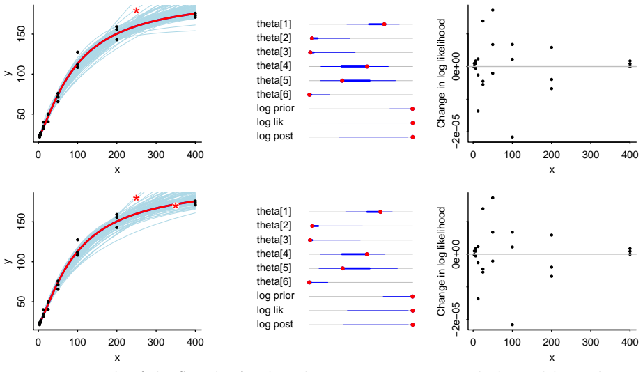
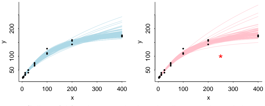
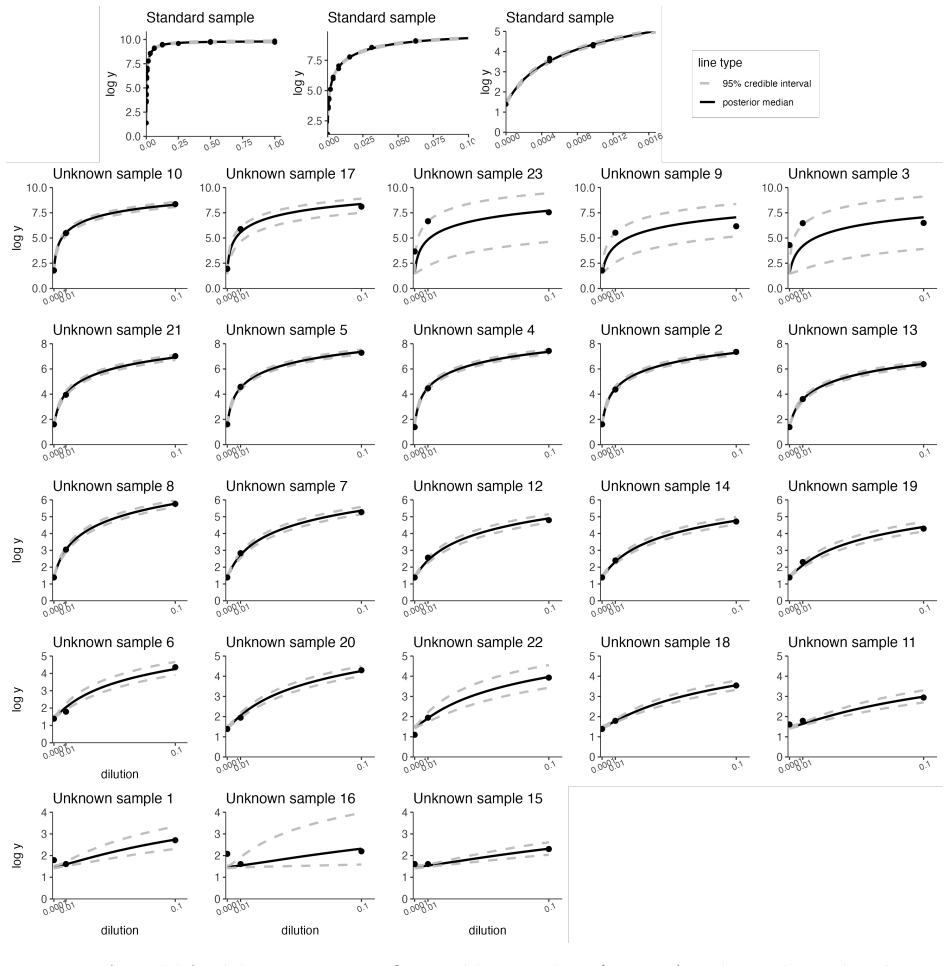
- Four-parameter models fitted to dilution-assay data become easier to tune because large residuals produce an audible cue.
- Cosmological parameter fits sensitive to Big Bang model values gain real-time auditory confirmation of alignment with observations.
- Nonparametric Gaussian process fits to temperature series allow users to hear when local adjustments create excess discrepancy.
Where Pith is reading between the lines
- The same principle could be applied to other sensory channels, such as vibration or color shifts, when auditory output is impractical.
- Embedding the feedback in standard statistical software might lower the barrier for non-statisticians to perform informal model checks.
- The method might be extended to higher-dimensional parameter spaces by mapping multiple discrepancy measures to different sound attributes.
Load-bearing premise
That the generated squeal will be noticeable and informative enough to help users detect misfits during real-time curve adjustment.
What would settle it
A user study in which participants adjust curves to minimize misfit with and without the squeal, then measure whether the squeal version produces systematically better final fits or faster detection of obvious mismatches.
Figures


read the original abstract
We introduce a method for visual and auditory feedback when exploring the fit of a model to data. Starting with a best-fit curve fit to data, the user can drag the curve to a new position and the computer will emit a squeal, becoming louder and more unpleasant as the discrepancy between curve and data increases. We demonstrate with four examples: a two-parameter curve fit to golf putting data, a four-parameter curve fit to dilution assays, a fit to cosmological data sensitive to the parameters of the Big Bang model, and a nonparametric Gaussian process fit to temperature readings.
Editorial analysis
A structured set of objections, weighed in public.
Referee Report
Summary. The paper introduces 'The Squealer', a method for visual and auditory feedback when exploring model fits to data. Starting from a best-fit curve, users drag the curve and receive a squeal whose volume and unpleasantness increase with growing discrepancy to the data points. The approach is illustrated via four examples: a two-parameter fit to golf putting data, a four-parameter fit to dilution assays, a cosmological fit sensitive to Big Bang parameters, and a nonparametric Gaussian process fit to temperature data.
Significance. If the chosen audio mapping can be shown to improve misfit detection, the technique could provide a practical multimodal aid for interactive model exploration in data analysis. The manuscript presents a direct conceptual proposal with no self-referential derivations or fitted quantities, and the four examples serve only as illustrations rather than tests of efficacy.
major comments (1)
- [Abstract] Abstract: the central claim that the squealing feedback 'meaningfully aids' interactive exploration and misfit detection rests on an untested assumption; the four examples demonstrate only the mapping from discrepancy to sound properties and supply no quantitative metrics, error analysis, user testing, or visual-only baseline comparisons.
minor comments (1)
- The term 'sensification' in the title is not defined or motivated in the provided text and may require a brief explanation for readers outside visualization or HCI communities.
Simulated Author's Rebuttal
We thank the referee for the detailed review. The manuscript presents a conceptual proposal for an auditory feedback technique, with the examples serving strictly as illustrations rather than efficacy tests. We address the single major comment below.
read point-by-point responses
-
Referee: [Abstract] Abstract: the central claim that the squealing feedback 'meaningfully aids' interactive exploration and misfit detection rests on an untested assumption; the four examples demonstrate only the mapping from discrepancy to sound properties and supply no quantitative metrics, error analysis, user testing, or visual-only baseline comparisons.
Authors: We agree there is no user testing, quantitative metrics, or baseline comparisons in the manuscript; the four examples illustrate application of the discrepancy-to-sound mapping across contexts (golf putting, dilution assays, cosmology, Gaussian processes) but do not evaluate performance gains. The provided abstract introduces the method and notes demonstration via examples without asserting empirical superiority. We will revise the abstract and introduction to explicitly frame the work as a conceptual proposal and remove any phrasing that could be read as claiming meaningful aid, thereby aligning the text with the illustrative scope. revision: partial
Circularity Check
No circularity: direct interface proposal without derivations or self-referential fits
full rationale
The paper introduces an auditory-visual feedback interface for model exploration but contains no equations, parameter fits, predictions, or derivations. Its central contribution is a proposed mapping from curve-data discrepancy to sound intensity, demonstrated via four qualitative examples. No load-bearing step reduces to a self-definition, fitted input renamed as prediction, or self-citation chain; the work is self-contained as a methodological suggestion with no mathematical claims that could be circular.
Axiom & Free-Parameter Ledger
Reference graph
Works this paper leans on
-
[1]
A unified pseudo-$C_\ell$ framework
Alonso, David, Javier Sanchez, and Anˇ ze Slosar (2019). “A unified pseudo-C ℓ framework”. In: Monthly Notices of the Royal Astronomical Society484, pp. 4127–4151.doi:10.1093/mnras/ stz093. eprint:1809.09603
work page internal anchor Pith review Pith/arXiv arXiv doi:10.1093/mnras/ 2019
-
[2]
Radical Compression of Cosmic Microwave Background Data
Bond, J. R., A. H. Jaffe, and L. Knox (2000). “Radical compression of cosmic microwave background data”. In:Astrophysical Journal533, p. 19.doi:10.1086/308625. eprint:astro-ph/9808264
work page internal anchor Pith review Pith/arXiv arXiv doi:10.1086/308625 2000
-
[3]
The sound of science
Bornmann, Lutz (2024). “The sound of science”. In:EMBO Reports25, pp. 3743–3747
2024
-
[4]
Two simple putting models in golf
Broadie, Mark (2018). “Two simple putting models in golf”. In:https://statmodeling.stat. columbia.edu/wp-content/uploads/2019/03/putt_models_20181017.pdf. Day´ e, Christian and Alberto de Campo (2006). “Sounds sequential: sonification in the social sci- ences”. In:Interdisciplinary Science Reviews31, pp. 349–364
2018
-
[5]
San Diego: Academic Press
Dodelson, Scott (2003).Modern Cosmology. San Diego: Academic Press
2003
-
[6]
Exploratory data analysis for complex models (with discussion)
Gelman, Andrew (2004). “Exploratory data analysis for complex models (with discussion)”. In: Journal of Computational and Graphical Statistics13, pp. 755–787
2004
-
[7]
Model building and expansion for golf putting
Gelman, Andrew (2019). “Model building and expansion for golf putting”. In:Stan Case Studies 6.https://mc-stan.org/users/documentation/case-studies/golf.html. 17
2019
-
[8]
The typical set and its relevance to Bayesian computation
Gelman, Andrew (2020). “The typical set and its relevance to Bayesian computation”. In:Statisti- cal Modeling, Causal Inference, and Social Science. 2 Aug.https : / / statmodeling . stat . columbia . edu / 2020 / 08 / 02 / the - typical - set - and - its - relevance - to - bayesian - computation/
2020
-
[9]
Bayesian analysis of serial dilu- tion assays
Gelman, Andrew, Ginger Chew, and Michael Shnaidman (2004). “Bayesian analysis of serial dilu- tion assays”. In:Biometrics60, pp. 407–417
2004
-
[10]
From visualization to sensification
Gelman, Andrew and S. Gwynn Sturdevant (2023). “From visualization to sensification”. In:Amstat News547, pp. 18–19
2023
-
[11]
(2026).Bayesian Workflow
Gelman, Andrew, Aki Vehtari, Richard McElreath, et al. (2026).Bayesian Workflow. London: CRC Press
2026
-
[12]
Hivon, E., K. M. G´ orski, C. B. Netterfield, B. P. Crill, S. Prunet, and F. Hansen (2002). “MASTER of the cosmic microwave background anisotropy power spectrum: A fast method for statistical analysis of large and complex cosmic microwave background data sets”. In:Astrophysical Jour- nal567, p. 2.doi:10.1086/338126. eprint:astro-ph/0105302
work page internal anchor Pith review Pith/arXiv arXiv doi:10.1086/338126 2002
-
[13]
The Physics of Microwave Background Anisotropies
Hu, Wayne, Naoshi Sugiyama, and Joseph Silk (1997). “The physics of microwave background anisotropies”. In:Nature386, pp. 37–43.doi:10.1038/386037a0. eprint:astro-ph/9504057
work page internal anchor Pith review Pith/arXiv arXiv doi:10.1038/386037a0 1997
-
[14]
Planck 2018 results. V. CMB power spectra and likelihoods
Liu, Jun S. and Rong Chen (1998). “Sequential Monte Carlo methods for dynamic systems”. In: Journal of the American Statistical Association93, pp. 1032–1044. Planck Collaboration, N. Aghanim, Y. Akrami, M. Ashdown, et al. (2020a). “Planck 2018 results. V. CMB power spectra and likelihoods”. In:Astronomy & Astrophysics641, A5.doi:10.1051/ 0004-6361/2018363...
work page internal anchor Pith review Pith/arXiv arXiv doi:10.1051/0004- 1998
-
[15]
Rasmussen, Carl Edward and Christopher K. I. Williams (2005).Gaussian Processes for Machine Learning. MIT Press
2005
-
[16]
Sturdevant, S. Gwynn, A. Jonathan R. Godfrey, and Andrew Gelman (2022). “Delivering data differently”. In:https://arxiv.org/abs/2204.10854
arXiv 2022
-
[17]
Exploratory model analysis with R and GGobi
Wickham, Hadley (2006). “Exploratory model analysis with R and GGobi”. In:https://had.co. nz/model-vis/2007-jsm.pdf
2006
-
[18]
Visualizing statistical models: Re- moving the blindfold
Wickham, Hadley, Dianne Cook, and Heike Hofmann (2015). “Visualizing statistical models: Re- moving the blindfold”. In:Statistical Analysis and Data Mining8, pp. 203–225. 18
2015
discussion (0)
Sign in with ORCID, Apple, or X to comment. Anyone can read and Pith papers without signing in.