Data-Based Dynamical Systems Reconstruction: An Adequacy/Reliability Test
Pith reviewed 2026-06-25 21:38 UTC · model grok-4.3
The pith
A two-step test validates reconstructions of stochastic dynamical systems from noisy data without arbitrary thresholds.
A machine-rendered reading of the paper's core claim, the machinery that carries it, and where it could break.
Core claim
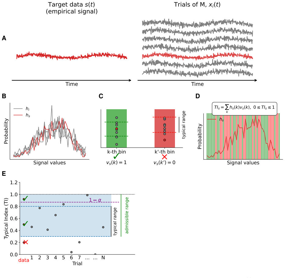
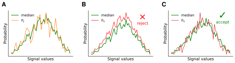
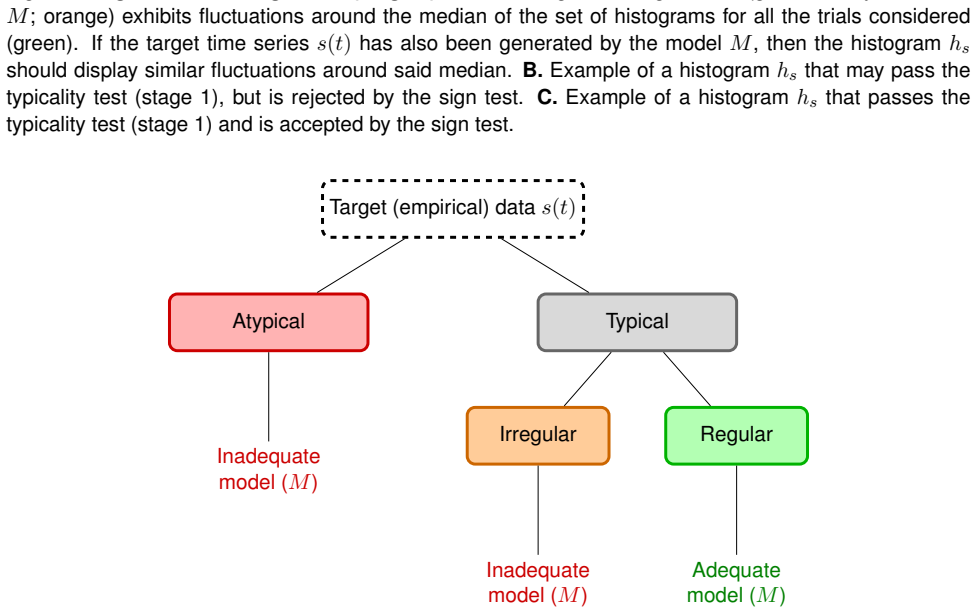
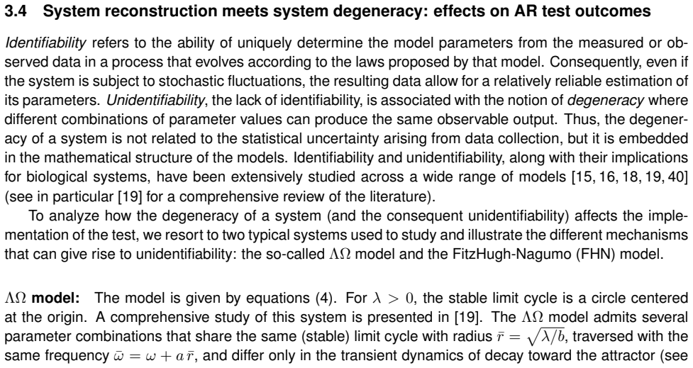
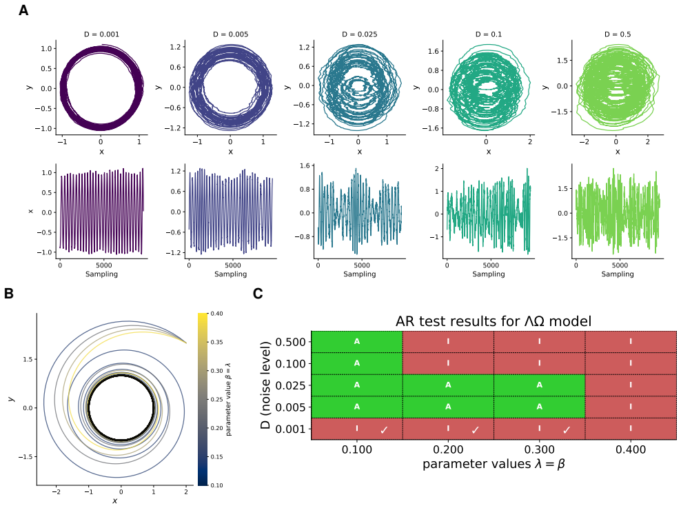
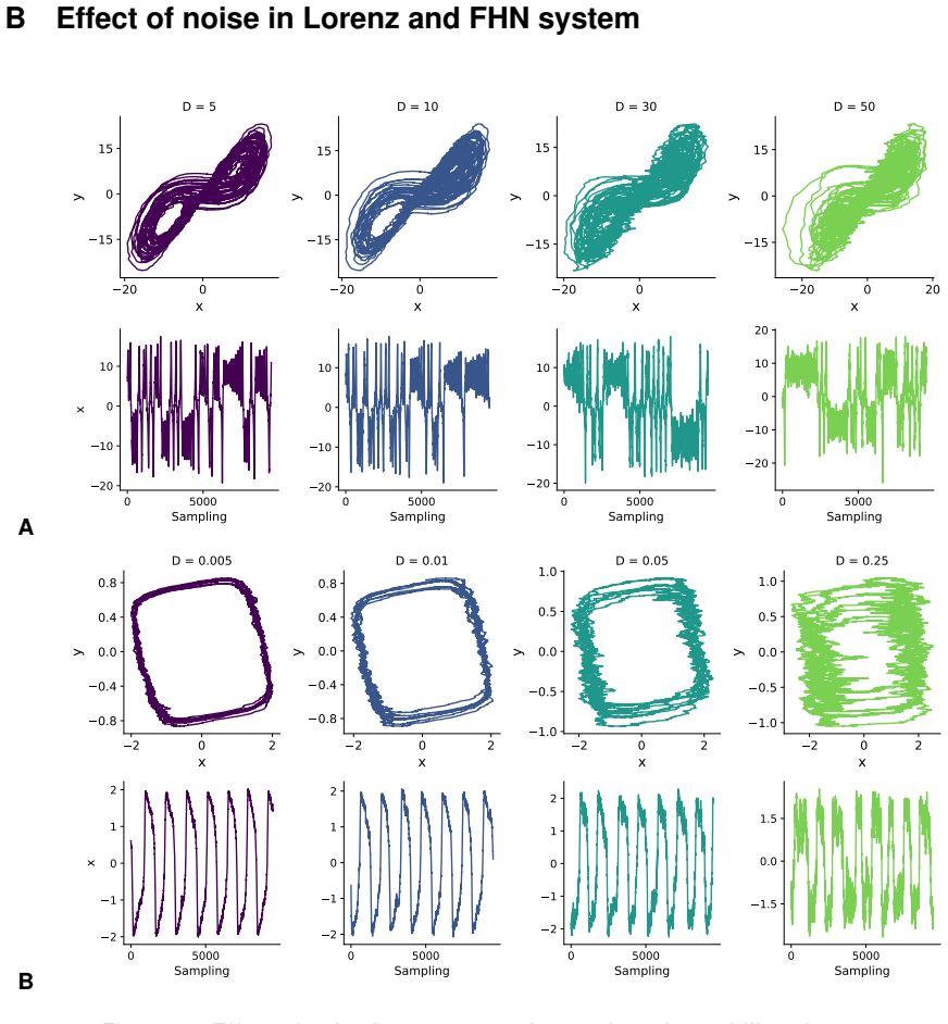
Standard criteria based solely on the loss function or deterministic metrics are insufficient for validating stochastic system reconstructions from noisy data. A two-step test provides a general assessment of reconstruction adequacy and reliability without arbitrary error-tolerance thresholds, subject to constraints imposed by system degeneracy, non-identifiability, and intrinsic stochastic features.
What carries the argument
The two-step test for assessing reconstruction adequacy and reliability.
If this is right
- Reconstructions of stochastic dynamics can be evaluated for adequacy without depending on user-chosen error thresholds.
- Validation remains possible in the presence of noise and stochasticity where deterministic metrics do not apply.
- The test explicitly accounts for cases where multiple models fit the data due to non-identifiability.
- Assessment is constrained rather than universally applicable when degeneracy is present.
Where Pith is reading between the lines
- The test could guide validation protocols in fields that routinely reconstruct stochastic models from time-series observations.
- It suggests a separation between deterministic and stochastic validation practices that may extend to other data-driven modeling tasks.
- Further work could test whether the two-step procedure distinguishes reconstructions that match low-order statistics but differ in higher-order dynamics.
Load-bearing premise
The two-step test can provide a general assessment of reconstruction adequacy even when system degeneracy, non-identifiability, and intrinsic stochastic features are present.
What would settle it
A known inadequate reconstruction that passes the two-step test while failing to match the original system's statistical behavior in new simulations, or an adequate reconstruction rejected by the test.
Figures


read the original abstract
In this work, we address the problem of validating the reconstruction of a stochastic system from noisy data. We demonstrate the limitations of criteria based solely on the loss function or on standard metrics used for reconstructing deterministic dynamics. We also propose an exploratory approach, based on a two-step test, which allows for a general assessment of the reconstruction without relying on arbitrary error-tolerance thresholds. However, we discuss how system degeneracy and non-identifiability, together with features intrinsic to stochastic dynamics, impose certain constraints on the application of this test.
Editorial analysis
A structured set of objections, weighed in public.
Referee Report
Summary. The manuscript addresses validating the reconstruction of stochastic systems from noisy data. It demonstrates limitations of loss-function criteria and standard metrics for deterministic dynamics. It proposes an exploratory two-step test for general assessment of reconstruction adequacy/reliability without arbitrary error-tolerance thresholds, while discussing constraints arising from system degeneracy, non-identifiability, and intrinsic stochastic features.
Significance. If the two-step test can be shown to deliver threshold-free assessment while respecting the stated constraints on degeneracy and non-identifiability, the work would supply a useful methodological contribution to data-driven stochastic modeling. The explicit acknowledgment of limitations is a positive feature.
major comments (2)
- [Abstract] Abstract: the two-step test is asserted to enable 'general assessment ... without relying on arbitrary error-tolerance thresholds,' yet no description of the test steps, no equations, no algorithm, and no worked example appear in the provided text, preventing evaluation of whether the claim holds or whether the test is independent of its own outputs.
- [Abstract] Abstract: the weakest assumption—that the test remains valid 'even when system degeneracy, non-identifiability, and intrinsic stochastic features are present'—is stated but not supported by any derivation, counter-example, or numerical demonstration, leaving the central claim unsubstantiated.
Simulated Author's Rebuttal
We thank the referee for the careful reading of our manuscript and for identifying points where the abstract's claims require stronger support in the presentation. We address each major comment below.
read point-by-point responses
-
Referee: [Abstract] Abstract: the two-step test is asserted to enable 'general assessment ... without relying on arbitrary error-tolerance thresholds,' yet no description of the test steps, no equations, no algorithm, and no worked example appear in the provided text, preventing evaluation of whether the claim holds or whether the test is independent of its own outputs.
Authors: The abstract summarizes the contribution at a high level, while the full manuscript (Sections 2–3) contains the explicit description of the two-step test, the associated equations, the algorithmic procedure, and numerical worked examples. To improve self-contained evaluation from the abstract, we will revise it to include a concise outline of the two steps and a reference to the supporting demonstrations in the body. revision: yes
-
Referee: [Abstract] Abstract: the weakest assumption—that the test remains valid 'even when system degeneracy, non-identifiability, and intrinsic stochastic features are present'—is stated but not supported by any derivation, counter-example, or numerical demonstration, leaving the central claim unsubstantiated.
Authors: The manuscript discusses the constraints arising from degeneracy, non-identifiability, and intrinsic stochasticity and illustrates the test's behavior in such regimes through examples. We agree that an explicit derivation or additional targeted demonstrations would better substantiate the claim of validity under these conditions. We will expand the discussion section with a dedicated paragraph providing this support. revision: yes
Circularity Check
No significant circularity detected
full rationale
The provided abstract and context contain no equations, fitted parameters, self-citations, or derivation steps that could be inspected for reduction to inputs by construction. The proposal of a two-step test is stated at a high level without any technical details, ansatzes, or load-bearing assumptions that match the enumerated circularity patterns. The manuscript is therefore self-contained against external benchmarks on the basis of the given text, with no evidence of self-definitional claims, fitted inputs renamed as predictions, or uniqueness imported via citation.
Axiom & Free-Parameter Ledger
Reference graph
Works this paper leans on
-
[1]
Training excitatory-inhibitory recurrent neural networks for cognitive tasks: a simple and flexible framework.PLoS computational biology, 12(2):e1004792, 2016
H Francis Song, Guangyu R Y ang, and Xiao-Jing Wang. Training excitatory-inhibitory recurrent neural networks for cognitive tasks: a simple and flexible framework.PLoS computational biology, 12(2):e1004792, 2016
2016
-
[2]
Daniel Durstewitz. A state space approach for piecewise-linear recurrent neural networks for identifying computational dynamics from neural measurements.PLoS computational biology, 13(6):e1005542, 2017
2017
-
[3]
Identifying non- linear dynamical systems via generative recurrent neural networks with applications to fMRI.PLoS computational biology, 15(8):e1007263, 2019
Georgia Koppe, Hazem Toutounji, Peter Kirsch, Stefanie Lis, and Daniel Durstewitz. Identifying non- linear dynamical systems via generative recurrent neural networks with applications to fMRI.PLoS computational biology, 15(8):e1007263, 2019
2019
-
[4]
Reconstructing computational system dy- namics from neural data with recurrent neural networks.Nature Reviews Neuroscience, 24(11):693– 710, 2023
Daniel Durstewitz, Georgia Koppe, and Max Ingo Thurm. Reconstructing computational system dy- namics from neural data with recurrent neural networks.Nature Reviews Neuroscience, 24(11):693– 710, 2023
2023
-
[5]
Multimodal teacher forcing for reconstructing nonlinear dynamical systems
Manuel Brenner, Georgia Koppe, and Daniel Durstewitz. Multimodal teacher forcing for reconstructing nonlinear dynamical systems. InWhen Machine Learning meets Dynamical Systems: Theory and Applications, 2023
2023
-
[6]
Daniel Kramer, Philine Lou Bommer, Carlo Tombolini, Georgia Koppe, and Daniel Durstewitz. Recon- structing nonlinear dynamical systems from multi-modal time series.arXiv preprint arXiv:2111.02922, 2021. 20
arXiv 2021
-
[7]
Time adaptive optimal transport: A framework of time series similarity measure.IEEE Access, 8:149764–149774, 2020
Zheng Zhang, Ping Tang, and Thomas Corpetti. Time adaptive optimal transport: A framework of time series similarity measure.IEEE Access, 8:149764–149774, 2020
2020
-
[8]
Guangyu R. Y ang H. Francis Song and Xiao-Jing Wang. Training excitatory-inhibitory recurrent neural networks for cognitive tasks: A simple and flexible framework.PLoS Comput Biol, 12(2), 2016
2016
-
[9]
Modern koopman theory for dynamical systems.arXiv preprint arXiv:2102.12086, 2021
Steven L Brunton, Marko Budiši ´c, Eurika Kaiser, and J Nathan Kutz. Modern koopman theory for dynamical systems.arXiv preprint arXiv:2102.12086, 2021
arXiv 2021
-
[10]
MIT Press, 2016
Ian Goodfellow, Y oshua Bengio, and Aaron Courville.Deep Learning. MIT Press, 2016
2016
-
[11]
Detecting strange attractors in turbulence
Floris Takens. Detecting strange attractors in turbulence. InDynamical Systems and Turbulence, Warwick 1980: proceedings of a symposium held at the University of Warwick 1979/80, pages 366–
1980
-
[12]
Approximation by superpositions of a sigmoidal function.Mathematics of control, signals and systems, 2(4):303–314, 1989
George Cybenko. Approximation by superpositions of a sigmoidal function.Mathematics of control, signals and systems, 2(4):303–314, 1989
1989
-
[13]
Encyclopedia of distances
Michel Marie Deza and Elena Deza. Encyclopedia of distances. InEncyclopedia of distances, pages 1–583. Springer, 2009
2009
-
[14]
Christoph Jürgen Hemmer, Manuel Brenner, Florian Hess, and Daniel Durstewitz. Optimal recurrent network topologies for dynamical systems reconstruction.arXiv preprint arXiv:2406.04934, 2024
arXiv 2024
-
[15]
On structural identifiability.Mathematical biosciences, 7(3- 4):329–339, 1970
Ror Bellman and Karl Johan Åström. On structural identifiability.Mathematical biosciences, 7(3- 4):329–339, 1970
1970
-
[16]
Claudio Cobelli and Joseph J Distefano 3rd. Parameter and structural identifiability concepts and ambiguities: a critical review and analysis.American Journal of Physiology-Regulatory, Integrative and Comparative Physiology, 239(1):R7–R24, 1980
1980
-
[17]
Similar network activity from disparate circuit parame- ters.Nature neuroscience, 7(12):1345–1352, 2004
Astrid A Prinz, Dirk Bucher, and Eve Marder. Similar network activity from disparate circuit parame- ters.Nature neuroscience, 7(12):1345–1352, 2004
2004
-
[18]
Structural and practical identifiability analysis of partially observed dynam- ical models by exploiting the profile likelihood.Bioinformatics, 25(15):1923–1929, 2009
Andreas Raue, Clemens Kreutz, Thomas Maiwald, Julie Bachmann, Marcel Schilling, Ursula Kling- müller, and Jens Timmer. Structural and practical identifiability analysis of partially observed dynam- ical models by exploiting the profile likelihood.Bioinformatics, 25(15):1923–1929, 2009
1923
-
[19]
Parameter estimation in the age of degeneracy and unidentifiability.Mathematics, 10(2):170, 2022
Dylan Lederman, Raghav Patel, Omar Itani, and Horacio G Rotstein. Parameter estimation in the age of degeneracy and unidentifiability.Mathematics, 10(2):170, 2022
2022
-
[20]
Exploratory data analysis.Reading/Addison-Wesley, 1977
John W Tukey. Exploratory data analysis.Reading/Addison-Wesley, 1977
1977
-
[21]
john wiley & sons, 1999
William Jay Conover.Practical nonparametric statistics, volume 350. john wiley & sons, 1999
1999
-
[22]
The double scroll family.IEEE transac- tions on circuits and systems, 33(11):1072–1118, 1986
LEONO Chua, Motomasa Komuro, and Takashi Matsumoto. The double scroll family.IEEE transac- tions on circuits and systems, 33(11):1072–1118, 1986
1986
-
[23]
A chaotic attractor from chua’s circuit.IEEE transactions on circuits and systems, 31(12):1055–1058, 2003
Takashi Matsumoto. A chaotic attractor from chua’s circuit.IEEE transactions on circuits and systems, 31(12):1055–1058, 2003
2003
-
[24]
Edward N. Lorenz. Deterministic nonperiodic flow.Journal of the Atmospheric Sciences, 20(2):130– 141, 1963
1963
-
[25]
Chapman and Hall/CRC, 2024
Steven H Strogatz.Nonlinear dynamics and chaos: with applications to physics, biology, chemistry, and engineering. Chapman and Hall/CRC, 2024
2024
-
[26]
Thresholds and plateaus in the hodgkin-huxley nerve equations.The Journal of general physiology, 43(5):867–896, 1960
Richard Fitzhugh. Thresholds and plateaus in the hodgkin-huxley nerve equations.The Journal of general physiology, 43(5):867–896, 1960. 21
1960
-
[27]
Fitzhugh–nagumo model
William Erik Sherwood. Fitzhugh–nagumo model. InEncyclopedia of Computational Neuroscience, pages 1439–1449. Springer, 2022
2022
-
[28]
Princeton University Press, 1988
Leon Glass and Michael C Mackey.From clocks to chaos: The rhythms of life. Princeton University Press, 1988
1988
-
[29]
MIT press, 2007
Eugene M Izhikevich.Dynamical systems in neuroscience. MIT press, 2007
2007
-
[30]
Springer, 2010
Bard Ermentrout and David M Terman.Mathematical foundations of neuroscience, volume 35. Springer, 2010
2010
-
[31]
L. D. Landau. On the problem of turbulence.Dokl. Akad. Nauk SSSR, 44(8):339–349, 1944
1944
-
[32]
J. T. Stuart. On the non-linear mechanics of hydrodynamic stability.Journal of Fluid Mechanics, 4(1):1–21, 1958
1958
-
[33]
Implementation of chua’s circuit with a cubic nonlinearity.IEEE Transactions on Circuits and Systems I: Fundamental Theory and Applications, 41(12):934–941, 1994
Guo-Qun Zhong. Implementation of chua’s circuit with a cubic nonlinearity.IEEE Transactions on Circuits and Systems I: Fundamental Theory and Applications, 41(12):934–941, 1994
1994
-
[34]
Lorenz equation and chua’s equation.Interna- tional Journal of Bifurcation and Chaos, 6(12b):2443–2489, 1996
Ladislav Pivka, Chai Wah Wu, and Anshan Huang. Lorenz equation and chua’s equation.Interna- tional Journal of Bifurcation and Chaos, 6(12b):2443–2489, 1996
1996
-
[35]
Transformation of relu-based recurrent neural networks from discrete-time to continuous-time
Zahra Monfared and Daniel Durstewitz. Transformation of relu-based recurrent neural networks from discrete-time to continuous-time. InInternational Conference on Machine Learning, pages 6999–
-
[36]
Cambridge university press, 2003
Endre Süli and David F Mayers.An introduction to numerical analysis. Cambridge university press, 2003
2003
-
[37]
Stochastic runge-kutta algorithms
Rebecca L Honeycutt. Stochastic runge-kutta algorithms. i. white noise.Physical Review A, 45(2):600, 1992
1992
-
[38]
Reconstructing computational system dy- namics from neural data with recurrent neural networks.Nature Reviews Neuroscience, 24:693–710, November 2023
Daniel Durstewitz, Georgia Koppe, and Max Ingo Thurm. Reconstructing computational system dy- namics from neural data with recurrent neural networks.Nature Reviews Neuroscience, 24:693–710, November 2023
2023
-
[39]
Reconstruction, forecasting, and stability of chaotic dynamics from partial data.Chaos: An Interdisciplinary Journal of Nonlinear Science, 33(9), 2023
Elise Özalp, Georgios Margazoglou, and Luca Magri. Reconstruction, forecasting, and stability of chaotic dynamics from partial data.Chaos: An Interdisciplinary Journal of Nonlinear Science, 33(9), 2023
2023
-
[40]
Global identifiability of nonlinear models of biological systems.IEEE Transactions on biomedical engineering, 48(1):55–65, 2002
Stefania Audoly, Giuseppina Bellu, Leontina D’Angio, Maria Pia Saccomani, and Claudio Cobelli. Global identifiability of nonlinear models of biological systems.IEEE Transactions on biomedical engineering, 48(1):55–65, 2002
2002
-
[41]
Stochastic resonance.Reviews of modern physics, 70(1):223, 1998
Luca Gammaitoni, Peter Hänggi, Peter Jung, and Fabio Marchesoni. Stochastic resonance.Reviews of modern physics, 70(1):223, 1998
1998
-
[42]
What can stochastic resonance do?Nature, 391(6665):344– 344, 1998
MI Dykman and Peter VE McClintock. What can stochastic resonance do?Nature, 391(6665):344– 344, 1998
1998
-
[43]
Stochastic res- onance in an electronic fitzhugh-nagumo model a.Annals of the New Y ork Academy of Sciences, 706(1):26–41, 1993
Frank Moss, John K Douglass, Lon Wilkens, David Pierson, and Eleni Pantazelou. Stochastic res- onance in an electronic fitzhugh-nagumo model a.Annals of the New Y ork Academy of Sciences, 706(1):26–41, 1993
1993
-
[44]
The detection threshold, noise and stochastic resonance in the fitzhugh-nagumo neuron model.Physics Letters A, 206(1-2):61–65, 1995
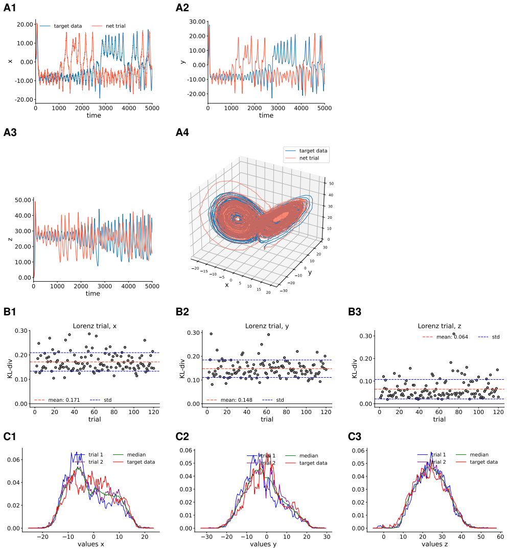
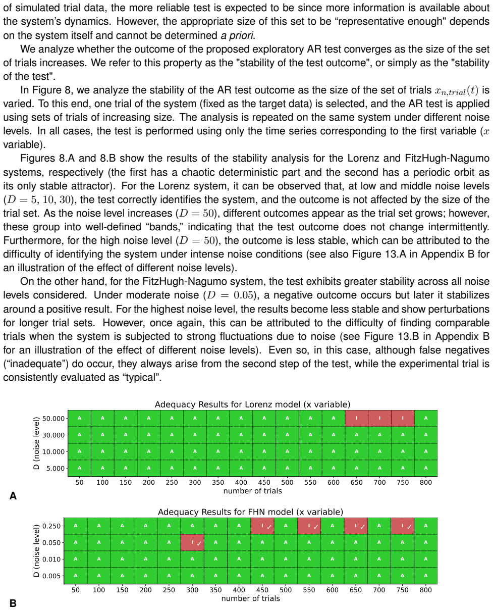
Xing Pei, Ken Bachmann, and Frank Moss. The detection threshold, noise and stochastic resonance in the fitzhugh-nagumo neuron model.Physics Letters A, 206(1-2):61–65, 1995. 22 A Inadequacy of measures to evaluate a putative reconstruction A1 A2 A3 0 20 40 60 80 100 120 trial 0.00 0.10 0.20 0.30 0.40Hellinged distance Lorenz trial, x mean: 0.369 std 0 20 4...
1995
discussion (0)
Sign in with ORCID, Apple, or X to comment. Anyone can read and Pith papers without signing in.