The Growing Pains of Frontier Models: When Leaderboards Stop Separating and What to Measure Next
Pith reviewed 2026-06-30 21:55 UTC · model grok-4.3
The pith
Frontier model capabilities cooperate across benchmarks rather than trade off, with cooperation strength varying fivefold by lab and permanent at pretraining.
A machine-rendered reading of the paper's core claim, the machinery that carries it, and where it could break.
Core claim
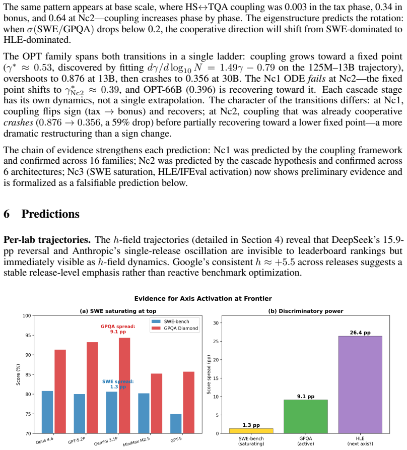
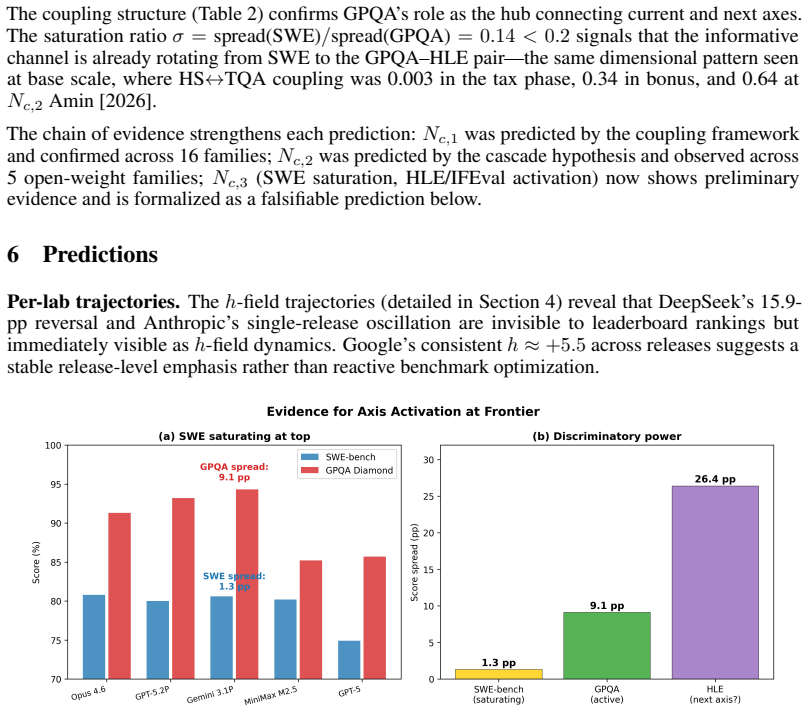
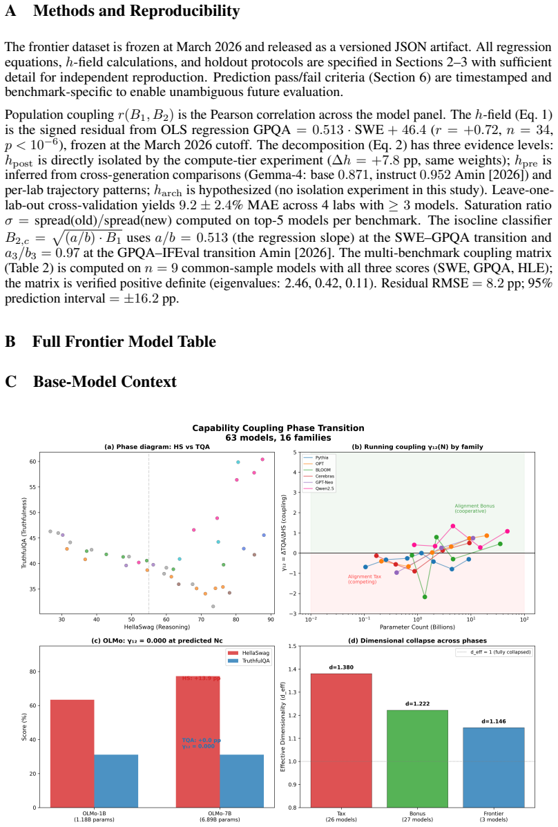
Across 34 models from 10 labs released 2024-2026, SWE-bench and GPQA Diamond scores correlate at r = +0.72. Per-lab slopes range from 1.15 (Google) to 0.23 (DeepSeek). The population regression line serves as an isocline phase boundary that classifies frontier models with the same sqrt((a/b)·B1) rule used at base scale and already flags mixed-phase behavior ahead of the next transition. Pretraining sets coupling near 0.871 while RLHF adds 0.081; pretraining shifts persist across releases, post-training shifts recover within one release, and inference compute alone moves the h-field by +7.8 pp.
What carries the argument
The h-field, the residual from the population regression trend between two benchmark scores, that isolates per-release capability emphasis and distinguishes pretraining from post-training effects.
If this is right
- Pretraining-level shifts remain fixed across multiple releases while post-training shifts reverse within one release.
- Inference compute alone can shift the h-field by +7.8 pp without any retraining.
- The same base-scale classifier identifies mixed-phase behavior at the frontier and flags two models below the GPQA-IFEval isocline.
- Five post-cutoff releases already fall inside the 95% prediction interval of the fitted trend.
- The h-field directly indicates whether retraining or waiting for inference scaling is the appropriate response.
Where Pith is reading between the lines
- The per-lab measurement-priority table could be used to select the next benchmark pair that best reveals a given lab's current emphasis.
- If the isocline continues to hold, the timing of the subsequent capability transition could be forecasted from the position of current models relative to the boundary.
- Applying the same decomposition to additional benchmark pairs might expose coupling patterns that are invisible from any single pair.
Load-bearing premise
That the population regression line fitted to the 34 models functions as a valid isocline phase boundary that correctly classifies frontier models and detects the next transition.
What would settle it
A new frontier model whose scores place it outside the 95% prediction interval of the population regression or whose lab-specific coupling slope deviates markedly from its prior releases.
Figures


read the original abstract
Leaderboards rank frontier models on independent axes but do not reveal whether capabilities reinforce or trade off across releases -- and at the frontier, this interaction is the more informative signal. We decompose paired SWE-bench and GPQA Diamond scores into a population coupling trend and per-release residual ($h$-field) that diagnoses capability emphasis from two public benchmark scores. Across 34 models from 10 labs (2024--2026), capabilities cooperate ($r = +0.72$, $p < 10^{-6}$), but cooperation varies systematically: per-lab coupling slopes span $5\times$ (Google $1.15$ vs. DeepSeek $0.23$), and labs pivot -- DeepSeek reversed from reasoning-rich to coding-first ($\Delta h = 15.9$~pp); Anthropic oscillates between coding excursions and recovery. The population regression serves as an isocline phase boundary: the same $\sqrt{(a/b)\cdot B_1}$ classifier that identifies the base-scale coupling transition [Amin, 2026] classifies frontier models and already detects mixed-phase behavior at the next transition (two models below the GPQA--IFEval isocline). The $h$-field is not just diagnostic -- it tells you what to change. Pretraining establishes coupling at $0.871$ while RLHF adds $0.081$ [Amin, 2026]: pretraining-level shifts are permanent (DeepSeek's four-release reversal persists), post-training shifts are reversible (Anthropic's three coding excursions each recover within one release), and inference compute alone shifts $h$ by $+7.8$~pp without retraining. Knowing which component dominates determines whether to retrain or wait. We provide a three-step diagnostic (locate, classify, predict), a per-lab measurement-priority table, and seven falsifiable predictions with timestamped criteria. Five post-cutoff releases fall within the 95\% prediction interval. Code, data, and an interactive dashboard: https://zehenlabs.com/cape/.
Editorial analysis
A structured set of objections, weighed in public.
Referee Report
Summary. The paper claims that paired SWE-bench and GPQA Diamond scores from 34 frontier models (10 labs, 2024–2026) can be decomposed into a population-level coupling trend and per-release h-field residuals. It reports positive capability cooperation (r = +0.72, p < 10^{-6}), 5× variation in per-lab coupling slopes, lab-specific pivots (e.g., DeepSeek Δh = 15.9 pp), and uses the population OLS line as an isocline phase boundary that extends the √((a/b)·B₁) classifier from prior work to classify models, detect mixed-phase behavior, and distinguish permanent pretraining shifts from reversible post-training shifts. The h-field is presented as actionable for deciding whether to retrain; the manuscript supplies a three-step diagnostic, a measurement-priority table, seven falsifiable predictions (five already verified post-cutoff), and public code/data/dashboard.
Significance. If the central decomposition and isocline hold, the work supplies a concrete, benchmark-driven method for interpreting capability interactions that leaderboards currently obscure, with direct implications for what labs should measure and when to intervene. The explicit falsifiable predictions, timestamped criteria, and release of code, data, and an interactive dashboard are strengths that enable immediate empirical scrutiny and extension by others.
major comments (3)
- [Abstract / isocline analysis] Abstract / isocline phase boundary: The claim that the OLS regression fitted to all 34 models functions as a valid isocline phase boundary (that correctly classifies frontier models and detects the next transition) is load-bearing for every downstream result on per-lab slopes, shift permanence, and mixed-phase detection. With only 10 labs and slopes spanning a 5× range, this aggregate line is vulnerable to being a mixture artifact; no leave-one-lab-out, bootstrap, or influence-function diagnostics are referenced, so the h-field residuals and the permanent/reversible distinction rest on an untested extrapolation from the base-scale classifier in [Amin, 2026].
- [Abstract] Abstract: The numerical attribution of coupling to pretraining (0.871) versus RLHF (0.081) and the √((a/b)·B₁) classifier itself are imported directly from [Amin, 2026] and then used to classify the current 34-model sample. The manuscript must state whether these quantities were re-estimated on the new data or assumed to transfer unchanged; the latter choice makes the h-field definition and the isocline boundary circular with respect to the cited prior work.
- [Predictions and verification] Predictions section: The assertion that five post-cutoff releases lie inside the 95 % prediction interval is presented as empirical support for the framework, yet the abstract supplies no model-selection criteria, regression specification, standard-error estimation, or multiple-comparison handling. Without these details the interval cannot be reproduced or stress-tested, weakening the falsifiability claim.
minor comments (2)
- The h-field residual and the precise functional form of the isocline boundary should be defined with an equation in the main text rather than relying solely on the citation to [Amin, 2026].
- Reported correlation and slope values would benefit from explicit confidence intervals or standard errors to convey sampling uncertainty.
Simulated Author's Rebuttal
We thank the referee for the constructive comments highlighting the need for robustness checks on the isocline and greater transparency on imported parameters and statistical details. We respond point-by-point below.
read point-by-point responses
-
Referee: [Abstract / isocline analysis] Abstract / isocline phase boundary: The claim that the OLS regression fitted to all 34 models functions as a valid isocline phase boundary (that correctly classifies frontier models and detects the next transition) is load-bearing for every downstream result on per-lab slopes, shift permanence, and mixed-phase detection. With only 10 labs and slopes spanning a 5× range, this aggregate line is vulnerable to being a mixture artifact; no leave-one-lab-out, bootstrap, or influence-function diagnostics are referenced, so the h-field residuals and the permanent/reversible distinction rest on an untested extrapolation from the base-scale classifier in [Amin, 2026].
Authors: We agree that the small number of labs raises legitimate concerns about mixture artifacts and that the absence of explicit robustness diagnostics weakens the isocline claim. In revision we will add leave-one-lab-out cross-validation of the OLS fit, bootstrap resampling to obtain confidence bands on the phase boundary, and influence-function analysis to identify any lab driving the line. These diagnostics will be reported alongside the main results to substantiate the h-field residuals and permanence distinction. revision: yes
-
Referee: [Abstract] Abstract: The numerical attribution of coupling to pretraining (0.871) versus RLHF (0.081) and the √((a/b)·B₁) classifier itself are imported directly from [Amin, 2026] and then used to classify the current 34-model sample. The manuscript must state whether these quantities were re-estimated on the new data or assumed to transfer unchanged; the latter choice makes the h-field definition and the isocline boundary circular with respect to the cited prior work.
Authors: The manuscript will be revised to state explicitly that the 0.871/0.081 attributions and the functional form of the classifier are taken unchanged from Amin et al. (2026) rather than re-estimated on the 34-model sample. We will add a dedicated paragraph discussing the transfer assumption, its implications for potential circularity in the h-field definition, and how the frontier data nevertheless provides an out-of-sample test of the earlier base-scale classifier. revision: yes
-
Referee: [Predictions and verification] Predictions section: The assertion that five post-cutoff releases lie inside the 95 % prediction interval is presented as empirical support for the framework, yet the abstract supplies no model-selection criteria, regression specification, standard-error estimation, or multiple-comparison handling. Without these details the interval cannot be reproduced or stress-tested, weakening the falsifiability claim.
Authors: We acknowledge that the current presentation lacks the necessary statistical details. The revised manuscript will specify the exact OLS regression equation (including any covariates), the model-selection procedure, the standard-error estimator (e.g., heteroskedasticity-robust), and the approach to multiple-comparison correction. These additions will allow independent reproduction and stress-testing of the 95 % prediction interval and the verification of the five post-cutoff releases. revision: yes
Circularity Check
Central √((a/b)·B₁) classifier, 0.871/0.081 attributions, and isocline phase boundary imported from self-citation [Amin, 2026]
specific steps
-
self citation load bearing
[Abstract]
"the same √((a/b)·B₁) classifier that identifies the base-scale coupling transition [Amin, 2026] classifies frontier models and already detects mixed-phase behavior at the next transition (two models below the GPQA--IFEval isocline). ... Pretraining establishes coupling at 0.871 while RLHF adds 0.081 [Amin, 2026]"
The load-bearing classifier, isocline concept, and attribution split (0.871 pretraining / 0.081 RLHF) are taken verbatim from the author's own prior paper and used to classify the current 34 models and diagnose h-field shifts, so the central phase-boundary claims and permanence/reversibility distinctions are equivalent to the self-cited inputs.
-
fitted input called prediction
[Abstract]
"The population regression serves as an isocline phase boundary: the same √((a/b)·B₁) classifier ... classifies frontier models"
The OLS regression line fitted across the 34 models is then treated as the valid isocline phase boundary that classifies those same models and extends the prior classifier, rendering the classification and transition detection statistically forced by the fit itself.
full rationale
The paper's derivation chain imports the core classifier √((a/b)·B₁), the isocline phase boundary concept, and the pretraining/RLHF decomposition values directly from the author's prior work [Amin, 2026] and applies them to classify and interpret the new 34-model dataset. The population OLS fit is then declared to serve as that same isocline, so downstream claims (per-lab slope variation, permanent vs. reversible shifts, mixed-phase detection) reduce to the self-cited result by construction rather than independent derivation here.
Axiom & Free-Parameter Ledger
free parameters (2)
- per-lab coupling slopes =
0.23 to 1.15
- h-field residuals =
e.g. +15.9 pp
axioms (2)
- domain assumption SWE-bench and GPQA Diamond represent independent capability axes whose interaction can be decomposed into coupling plus residual.
- ad hoc to paper The base-scale coupling transition classifier from prior work applies unchanged to frontier models.
invented entities (1)
-
h-field
no independent evidence
Forward citations
Cited by 2 Pith papers
-
Lying Is Just a Phase: The Hidden Alignment Transition in Language Model Scaling
Language models show a scale-dependent switch from anticorrelated to correlated reasoning-truthfulness coupling at a family-specific critical parameter count, with architecture and data choices shifting the transition point.
-
Lying Is Just a Phase: The Hidden Alignment Transition in Language Model Scaling
Language models exhibit a family-dependent phase transition at roughly 3.5 billion parameters, flipping the relationship between reasoning and truthfulness from anticorrelated to cooperative.
Reference graph
Works this paper leans on
-
[1]
When AI Benchmarks Plateau: A Systematic Study of Benchmark Saturation
Mubashara Akhtar, Anka Reuel, Prajna Soni, et al. When ai benchmarks plateau: A systematic study of benchmark saturation.arXiv preprint arXiv:2602.16763,
work page internal anchor Pith review Pith/arXiv arXiv
-
[3]
Lying Is Just a Phase: The Hidden Alignment Transition in Language Model Scaling
URLhttps://arxiv.org/abs/2605.18838. 11 Lluís Arola-Fernández and Lucas Lacasa. Effective theory of collective deep learning.Physical Review Research, 6:L042040,
work page internal anchor Pith review Pith/arXiv arXiv
-
[4]
Scaling Laws for Neural Language Models
Jared Kaplan, Sam McCandlish, Tom Henighan, Tom B Brown, Benjamin Chess, Rewon Child, Scott Gray, Alec Radford, Jeffrey Wu, and Dario Amodei. Scaling laws for neural language models. arXiv preprint arXiv:2001.08361,
work page internal anchor Pith review Pith/arXiv arXiv 2001
-
[5]
All regression equations, h-field calculations, and holdout protocols are specified in Sections 2–3 with sufficient detail for independent reproduction
12 A Methods and Reproducibility The frontier dataset is frozen at March 2026 and released as a versioned JSON artifact. All regression equations, h-field calculations, and holdout protocols are specified in Sections 2–3 with sufficient detail for independent reproduction. Prediction pass/fail criteria (Section
2026
-
[6]
The decomposition (Eq
is the signed residual from OLS regression GPQA= 0.513·SWE+ 46.4 (r= +0.72 , n= 34 , p <10 −6), frozen at the March 2026 cutoff. The decomposition (Eq
2026
-
[7]
Leave-one- lab-out cross-validation yields 9.2±2.4 % MAE across 4 labs with ≥3 models
has three evidence levels: hpost is directly isolated by the compute-tier experiment ( ∆h= +7.8 pp, same weights); hpre is inferred from cross-generation comparisons (Gemma-4: base 0.871, instruct 0.952 Amin [2026]) and per-lab trajectory patterns; harch is hypothesized (no isolation experiment in this study). Leave-one- lab-out cross-validation yields 9....
2026
-
[8]
Residual RMSE = 8.2 pp; 95% prediction interval=±16.2pp
is computed on n= 9 common-sample models with all three scores (SWE, GPQA, HLE); the matrix is verified positive definite (eigenvalues: 2.46, 0.42, 0.11). Residual RMSE = 8.2 pp; 95% prediction interval=±16.2pp. B Full Frontier Model Table C Base-Model Context Figure 5:Base-model foundation (from Amin [2026]).The coupling regime transition underlying CAPE...
2026
discussion (0)
Sign in with ORCID, Apple, or X to comment. Anyone can read and Pith papers without signing in.