REVIEW 4 major objections 5 minor 2 cited by
Neural Thermodynamic Laws for Large Language Model Training
T0 review · 4 major / 5 minor · reviewed 2026-08-15 · deepseek-v4-flash
Pith's one-line read LLM training is a thermodynamic process: the learning rate acts as temperature, and the thermal part of the final loss grows linearly with it.
desk verdict Clean toy-model thermodynamics with a well-tested 1/t decay rule; the GPT-2 confirmation is suggestive but not load-bearing, and the D-confound note reverses the sign of Fig. 4's slope. read the letter →
The pith
A machine-rendered reading of the paper's core claim, the machinery that carries it, and where it could break.
The reading
What carries the argument
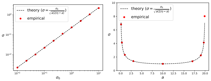
The river-valley toy model $\ell(x,y) = c(y) + \frac12 a(y)x^2$, with fast variable $x$ and slow variable $y$, is the load-bearing object. For fixed $y$ the fast coordinate equilibrates to a Gaussian of width $\sigma = d(\eta,\sigma_g)/\sqrt{a}$, and the key identity is that the thermal loss $\ell_f = \frac12 a\sigma^2 = C\eta$ is independent of sharpness $a$. This calculation carries the thermodynamic mapping: $\eta$ is temperature, $C$ is heat capacity, the exponential relaxation of $\ell_f$ toward $C\eta_B$ is thermal conduction, and the step-by-step minimization of $\sigma_{t+1}^2$ with respect to $\eta_t$ yields the optimal $1/t$ decay schedule.
What would settle it
Scan the final learning rate $\eta_{\min}$ while varying the decay-phase length (for example, 1k, 3k, and 10k steps): the thermodynamic claim predicts that the fitted slope in $\ell = 3.145 + 110\eta_{\min}$ stays the same whenever the decay is long enough for quasi-static annealing, whereas a slope that changes with decay length would show that the constant-$\ell_s$ assumption fails and the equipartition reading is unsupported.
Extended reading notes
Core claim
The central discovery is that the fast valley dynamics of stochastic gradient descent and sign descent converge to a Gaussian steady state whose width scales as $\sigma \approx \sqrt{\eta/(2a)}\,\sigma_g$ in the flat limit, so the averaged fast loss $\ell_f = \frac12 a\sigma^2 = C\eta$ is independent of the sharpness $a$. This is the neural analog of the equipartition theorem: every valley direction contributes the same thermal loss, so the total is $L_f = N C \eta$, with the learning rate acting as temperature and the slope $C$ as heat capacity. The paper then uses this identity to explain why the final validation loss of a GPT-style model is linear in the final learning rate, and derives the optimal decay schedule by choosing $\eta_t$ at each step to minimize the next Gaussian width, obtaining $\eta_t = (\eta/2)/(1 + t/t_h)$. The slow river dynamics is shown to feel an entropic force proportional to the gradient of $-\frac12 \log a$, so valleys that narrow along the river can trap the optimizer.
Load-bearing premise
The empirical identification of the fitted slope $110$ as purely thermal loss requires that the slow river loss $\ell_s$ does not change across the decay schedules, so that the measured final validation loss is a proxy for the thermal loss $\ell_f$; if $\ell_s$ shifts with $\eta_{\min}$, the inferred valley-direction count and the thermodynamic confirmation lose their quantitative meaning.
Editorial extensions
If this is right
- Final loss separates into a river part controlled by the learning-rate sum $D$, a thermal part controlled by the final learning rate $\eta_{\min}$, and two correction terms from entropic forces and incomplete annealing: $\ell_{\mathrm{final}} = \ell(D,\eta_{\min}) + \Delta_{\mathrm{entropic}} + \Delta_{\mathrm{anneal}}$.
- Because $1/\sigma_t^2$ grows as an arithmetic sequence under the optimal schedule, the thermal loss decays as $1/t$ and the learning rate as $\eta_t = (\eta/2)/(1+t/t_h)$, so $1/t$ decay is optimal for isotropic valleys rather than linear or cosine decay.
- The first decay step should jump from $\eta$ to roughly $\eta/2$; continuous learning-rate schedules that start decaying smoothly from $\eta$ are suboptimal because neither keeping $\eta$ nor dropping to $0$ decreases the variance.
- Decaying all the way to zero is suboptimal because reaching $\eta_{\min}=0$ would take infinite time; the decay time needed to reach a small $\eta_{\min}$ is bounded by $O(1/\eta_{\min})$, independent of the stable learning rate.
- Increasing the stable learning rate lowers the river loss by raising the learning-rate sum $D$ without requiring a longer decay phase, which is why a larger stable learning rate improves validation loss up to numerical stability limits.
Reading between the lines
- Extension: the inferred count $N \approx 5\times 10^6$ valley directions is a concrete microstate count; if the thermodynamic picture is right, the Hessian spectrum of a similarly trained GPT-style model should show roughly five million high-curvature directions, which an independent Hessian measurement could confirm.
- Extension: the equipartition law predicts a precise batch-size trade-off, because gradient noise scales as $\sigma_g \propto 1/\sqrt{B}$ for SGD, making the thermal slope $C$ scale as $1/B$ (or $1/\sqrt{B}$ for sign updates); scanning batch size at fixed $\eta_{\min}$ would test this prediction directly.
- Extension: the framework predicts that entropic trapping grows stronger as training proceeds and valleys sharpen, so the near-perfect loss-curve alignment seen in the early GPT experiment may fail at much larger compute budgets, which would be visible as a growing misalignment in learning-rate-sum plots.
Signed reviews
Editorial analysis
A structured set of objections, weighed in public.
Referee Report
Summary. The paper introduces Neural Thermodynamic Laws (NTL), a framework that maps stochastic optimization of large language models in a 'river-valley' loss landscape to thermodynamics. It analyzes a toy model with a fast quadratic valley direction x and a slow river direction y. With a fixed learning rate, the valley dynamics reach a Gaussian steady state whose average fast loss is linear in the learning rate and independent of curvature (equipartition), motivating an effective temperature T~η and a heat capacity C. During decay, the authors derive an optimal 1/t learning-rate schedule for the fast component. In the slow dynamics, the averaged fast loss produces an entropic force proportional to -∇ log a(y). The paper validates the optimal schedule in toy experiments and reports that GPT-2 pretraining validation loss is linear in the final learning rate η_min with slope 110, interpreted as N·C with N≈5×10^6 valley directions. It also draws analogies to the three laws of thermodynamics, Fourier's law, and entropic trapping, and gives practical guidance for WSD schedules.
Significance. The toy-model derivations in Sections 3–5 are internally consistent and exactly solvable, the toy experiments verify the predicted optimal decay schedule, and the framework yields falsifiable predictions (the linear ℓ_f–η relation, the 1/t schedule, and the dependence on the learning-rate sum D). These are genuine strengths. If the quantitative LLM result were validated, the paper would offer a significant mechanistic connection between optimizers and thermodynamics. However, the LLM evidence is currently too weak to support the claimed quantitative confirmation: a single small model, no error bars, a slope used to fit N rather than to test a pre-specified constant, an untested assumption about ℓ_s, and an unbridged application of SignGD theory to Adam. The significance is therefore conditional on the experimental identification being fixed.
major comments (4)
- [Sec. 3.3; Eq. (6); Figs. 2(b), 4] The identification of the fitted slope dℓ/dη_min = 110 with the thermal coefficient NC is confounded by slow-loss variation with the learning-rate sum D. In the WSD sweep, D = 0.6 (warmup) + 4.2 (stable) + 0.3 (decay) + 500 η_min = 5.1 + 500 η_min, so ΔD = 0.3 across η_min ∈ [0, 6×10^-4]. The paper's own Fig. 4 shows validation loss depending on D; using a slope of roughly 0.1 as read from that figure, ΔD = 0.3 predicts Δℓ_s ≈ 0.03, about half of the observed Δℓ ≈ 0.066. The statement in Sec. 3.3 that 'ℓ_s does not vary much across decay schedules' is therefore unsupported and conflicts with Eq. (6), which lists ℓ(D, η_min) as the dominant term. The slope 110 and the inferred N ≈ 5×10^6 are not identified unless D is held fixed or the ℓ_s(D) contribution is subtracted.
- [Sec. 3.3; Table 1; footnote 3] The quantitative comparison uses the SignGD steady-state coefficient L_f = N√(π/32)σ_g η, but the GPT-2 runs use Adam with finite β1 and β2 plus adaptive scaling, not SignGD. The footnote that SignGD is a special case of Adam when (β1, β2) = (0, 0) does not supply a bridging argument: standard Adam's update and noise properties differ. Without a stated and tested assumption that Adam has the same linear thermal-loss law and coefficient, the reported N is an interpretation of a fitted slope rather than a quantitative prediction. The estimate σ_g ≈ 7×10^-5 is also not documented; N is inversely proportional to σ_g, so this free parameter drives the headline number.
- [Sec. 6 vs. Sec. 3.3] The paper states that Δ_anneal ≈ 0 when the decay phase is at least 3k steps (Sec. 6), but the GPT-2 experiment in Fig. 2 uses a 1k-step cosine decay. By the paper's own criterion, the final losses in Fig. 2(b) may include a non-negligible annealing correction, so the identification ℓ ≈ ℓ_f(η_min) used to interpret the slope 110 is not supported. The experiment should either use a decay phase long enough for quasi-static equilibrium or explicitly model the annealing correction.
- [Sec. 3.3] The LLM evidence rests on a single GPT-2-small run per η_min value with no error bars or repeated seeds. The quantitative claim is a linear fit over a small number of points, with the linear regime selected post hoc; run-to-run variance could change the fitted slope substantially. Reporting means and standard errors over several seeds is necessary to support the claimed coefficient 110 and the resulting N.
minor comments (5)
- [Sec. 3.1] The text uses 'SignSGD' in the first paragraph but 'SignGD' throughout the rest of the paper; the terminology should be unified.
- [Sec. 5.2] In the definition of entropy, the slow-variable dependence is written with x (e.g., 'S(x) ∝ −1/2 log a(x)') even though a is a function of the slow variable y; this is confusing and should be corrected to a(y).
- [Table 1 and Sec. 4.1] The half-time t_h for SignGD is typeset with an ambiguous square-root expression; it should be written unambiguously (e.g., √(2π) σ_g/(aη)) to match the Appendix C derivation.
- [Sec. 3.3] The experiment description omits the number of data points in the linear fit, the validation split details, and the Adam hyperparameters (β1, β2, ε, weight decay); these details are needed for reproducibility.
- [Sec. 5.3] The claim that the three learning-rate curves 'align reasonably well' is judged visually; a quantitative alignment metric or residual reporting would strengthen the conclusion about entropic forces.
Circularity Check
Partial circularity: the GPT-2 thermal slope 110 is converted into the valley-direction count N by assuming the slow loss is ηmin-independent, while the paper's own Eq. (6) and Section 5 make the slow loss a function of the learning-rate sum D, which varies with ηmin in the same WSD sweep.
-
fitted input called prediction
[Section 3.3, GPT-2 experiment (Figure 2), with cross-reference to Section 6, Eq. (6).]
"Since the decay phase is short, we can assume that ℓs does not vary much across decay schedules. As a result, ℓ is representative of ℓf, and we measure that ℓ = 3.145 + 110ηmin. Comparing to the theoretical thermal loss ... we have N = 110/σg q 32/π ≈ 5×10^6 = 5M"
The slope 110 is turned into the theoretical parameter N, so the claimed confirmation of NTL is a fit, not a predictive test with a pre-specified constant. The identifying assumption that ℓs is constant across decay schedules is contradicted by the paper's own Eq. (6), ℓfinal = ℓ(D,ηmin) + Δentropic + Δanneal, and by Section 5's alignment of validation loss against the learning-rate sum D. In the 2k warmup + 7k stable + 1k cosine decay sweep, D ≈ 5.1 + 500ηmin, so D changes by ≈0.3 as ηmin goes from 0 to 6×10^-4; Figure 4 indicates Δℓs ≈ 0.1ΔD ≈ 0.03, roughly half of the observed Δℓ ≈ 0.066. Thus the measured 110 can be substantially a slow-loss artifact, and N ≈ 5×10^6 is not identified as the number of thermal valley directions.
full rationale
The toy-model derivations in Sections 3.1-3.2, 4.1, and 5.1 are self-contained: the Gaussian steady state, the flat-limit σ ∝ (η/a)^1/2, the equipartition-like cancellation of a in ℓf, the optimal 1/t decay, and the entropic force F_ent = -d^2 a'/2a are all derived from the stated SGD/SignGD dynamics without importing the target conclusions. The thermodynamic vocabulary (temperature T ∼ η, heat capacity C, entropy S) is an interpretive layer rather than a circular reduction; the entropy identification is additionally supported by the Gibbs entropy of the Gaussian, S_phy = -1/2 log a + const. The paper's self-citations (e.g., [7] FOCUS) appear only in a proof-of-concept appendix and are not load-bearing. The circularity is confined to the claimed quantitative LLM validation in Section 3.3: the linear slope is used to fit N, and the attribution of the whole slope to thermal loss rests on an 'assume ℓs does not vary' step that the paper's own Eq. (6) and Section 5 undercut. This is partial circularity, not complete; hence a score of 4 rather than 6 or higher.
Assumptions & free parameters
free parameters (3)
- slope of linear loss-ηmin fit =
110
- number of valley directions N =
≈5×10^6
- gradient noise scale σg =
≈7×10^-5
assumptions (7)
- domain assumption LLM loss landscape is a river-valley: flat river directions plus sharp valley directions.
- domain assumption The fast-direction loss is quadratic ℓf = ½a(y)x² and total loss decomposes additively ℓ = ℓs + ℓf.
- domain assumption Fast and slow dynamics decouple (timescale separation), so y can be treated as fixed in fast dynamics.
- domain assumption Gradient noise is Gaussian with variance σg² in the toy dynamics.
- domain assumption Flat limit aη << 1 holds for valley directions of interest.
- ad hoc to paper ℓs does not vary across decay schedules; measured total loss ℓ represents ℓf.
- domain assumption Adam optimizer dynamics in experiments are approximated by SignGD (or SGD) theory.
invented entities (2)
-
Effective temperature T ~ η
independent evidence
-
Entropic force F_ent = -d²/2 · a'/a
independent evidence
Cite this review
Pith. "Pith review of Neural Thermodynamic Laws for Large Language Model Training." pith.science (2026). https://pith.science/paper/JAJ7S2BT
@misc{pith2026250510559,
  author       = {Pith},
  title        = {Pith review of: Neural Thermodynamic Laws for Large Language Model Training},
  year         = {2026},
  howpublished = {\url{https://pith.science/paper/JAJ7S2BT}},
  note         = {Machine review of arXiv:2505.10559}
}
read the original abstract
Beyond neural scaling laws, little is known about the laws underlying large language models (LLMs). We introduce Neural Thermodynamic Laws (NTL) -- a new framework that offers fresh insights into LLM training dynamics. On the theoretical side, we demonstrate that key thermodynamic quantities (e.g., temperature, entropy, heat capacity, thermal conduction) and classical thermodynamic principles (e.g., the three laws of thermodynamics and the equipartition theorem) naturally emerge under river-valley loss landscape assumptions. On the practical side, this scientific perspective yields intuitive guidelines for designing learning rate schedules.
Figures


Figures from the paper (7 more)



Forward citations
Cited by 2 Pith papers
-
Falcon-H1: A Family of Hybrid-Head Language Models Redefining Efficiency and Performance
Falcon-H1 reports competitive benchmark scores for a 0.5B to 34B family of parallel hybrid attention/Mamba-2 models, claiming 2x to 4x parameter efficiency versus dense transformers.
-
Mpemba Effect in Large-Language Model Training Dynamics: A Minimal Analysis of the Valley-River model
The authors derive conditions under which a higher plateau learning rate accelerates LLM training convergence via the Mpemba effect, but the central derivative formula is incorrect.
Reference graph
Works this paper leans on
-
[1]
Bayesian learning via stochastic gradient langevin dynamics
Max Welling and Yee W Teh. Bayesian learning via stochastic gradient langevin dynamics. In Proceedings of the 28th international conference on machine learning (ICML-11) , pages 681–688. Citeseer, 2011
2011
-
[2]
Thermodynamics-inspired explanations of artificial intelli- gence
Shams Mehdi and Pratyush Tiwary. Thermodynamics-inspired explanations of artificial intelli- gence. Nature Communications, 15(1):7859, 2024
work page 2024
-
[3]
Statistical mechanics of learning
Andreas Engel. Statistical mechanics of learning . Cambridge University Press, 2001
work page 2001
-
[4]
Statistical mechanics of deep learning
Yasaman Bahri, Jonathan Kadmon, Jeffrey Pennington, Sam S Schoenholz, Jascha Sohl- Dickstein, and Surya Ganguli. Statistical mechanics of deep learning. Annual review of condensed matter physics, 11(1):501–528, 2020
work page 2020
-
[5]
Understanding warmup-stable-decay learning rates: A river valley loss landscape perspective
Kaiyue Wen, Zhiyuan Li, Jason Wang, David Hall, Percy Liang, and Tengyu Ma. Understanding warmup-stable-decay learning rates: A river valley loss landscape perspective. arXiv preprint arXiv:2410.05192, 2024
arXiv 2024
-
[6]
How noise affects the hessian spectrum in overparameterized neural networks
Mingwei Wei and David J Schwab. How noise affects the hessian spectrum in overparameterized neural networks. arXiv preprint arXiv:1910.00195, 2019
arXiv 1910
-
[7]
Focus: First order concentrated updating scheme
Yizhou Liu, Ziming Liu, and Jeff Gore. Focus: First order concentrated updating scheme. arXiv preprint arXiv:2501.12243, 2025
arXiv 2025
-
[8]
Minicpm: Unveiling the potential of small language models with scalable training strategies
Shengding Hu, Yuge Tu, Xu Han, Chaoqun He, Ganqu Cui, Xiang Long, Zhi Zheng, Yewei Fang, Yuxiang Huang, Weilin Zhao, et al. Minicpm: Unveiling the potential of small language models with scalable training strategies. arXiv preprint arXiv:2404.06395, 2024
arXiv 2024
Show all 34 references
-
[9]
Gra- dient descent on neural networks typically occurs at the edge of stability
Jeremy M Cohen, Simran Kaur, Yuanzhi Li, J Zico Kolter, and Ameet Talwalkar. Gra- dient descent on neural networks typically occurs at the edge of stability. arXiv preprint arXiv:2103.00065, 2021
2021 arXiv
-
[10]
Scaling laws and compute-optimal training beyond fixed training durations
Alex Hägele, Elie Bakouch, Atli Kosson, Leandro V on Werra, Martin Jaggi, et al. Scaling laws and compute-optimal training beyond fixed training durations. Advances in Neural Information Processing Systems, 37:76232–76264, 2024
2024
-
[11]
Andrej Karpathy. NanoGPT. https://github.com/karpathy/nanoGPT, 2022
2022
-
[12]
A multi-power law for loss curve prediction across learning rate schedules
Kairong Luo, Haodong Wen, Shengding Hu, Zhenbo Sun, Maosong Sun, Zhiyuan Liu, Kaifeng Lyu, and Wenguang Chen. A multi-power law for loss curve prediction across learning rate schedules. In The Thirteenth International Conference on Learning Representations , 2025
2025
-
[13]
modded-nanogpt
Jordan Keller. modded-nanogpt. https://github.com/KellerJordan/modded-nanogpt,
-
[14]
Implicit gradient regularization
David GT Barrett and Benoit Dherin. Implicit gradient regularization. arXiv preprint arXiv:2009.11162, 2020
2009 arXiv
-
[15]
The limiting dynamics of sgd: Modified loss, phase-space oscillations, and anomalous diffusion
Daniel Kunin, Javier Sagastuy-Brena, Lauren Gillespie, Eshed Margalit, Hidenori Tanaka, Surya Ganguli, and Daniel LK Yamins. The limiting dynamics of sgd: Modified loss, phase-space oscillations, and anomalous diffusion. Neural Computation, 36(1):151–174, 2023
2023
-
[16]
Stochastic collapse: How gra- dient noise attracts sgd dynamics towards simpler subnetworks.Advances in Neural Information Processing Systems, 36:35027–35063, 2023
Feng Chen, Daniel Kunin, Atsushi Yamamura, and Surya Ganguli. Stochastic collapse: How gra- dient noise attracts sgd dynamics towards simpler subnetworks.Advances in Neural Information Processing Systems, 36:35027–35063, 2023
2023
-
[17]
Stochastic gradient descent as approximate bayesian inference
Mandt Stephan, Matthew D Hoffman, David M Blei, et al. Stochastic gradient descent as approximate bayesian inference. Journal of Machine Learning Research, 18(134):1–35, 2017. 10
2017
-
[18]
A diffusion theory for deep learning dynamics: Stochastic gradient descent exponentially favors flat minima
Zeke Xie, Issei Sato, and Masashi Sugiyama. A diffusion theory for deep learning dynamics: Stochastic gradient descent exponentially favors flat minima. arXiv preprint arXiv:2002.03495, 2020
2002 arXiv
-
[19]
Direction matters: On the implicit bias of stochastic gradient descent with moderate learning rate
Jingfeng Wu, Difan Zou, Vladimir Braverman, and Quanquan Gu. Direction matters: On the implicit bias of stochastic gradient descent with moderate learning rate. arXiv preprint arXiv:2011.02538, 2020
2011 arXiv
-
[20]
Gradient descent maximizes the margin of homogeneous neural networks
Kaifeng Lyu and Jian Li. Gradient descent maximizes the margin of homogeneous neural networks. arXiv preprint arXiv:1906.05890, 2019
1906 arXiv
-
[21]
The implicit bias for adaptive optimization algorithms on homogeneous neural networks
Bohan Wang, Qi Meng, Wei Chen, and Tie-Yan Liu. The implicit bias for adaptive optimization algorithms on homogeneous neural networks. InInternational Conference on Machine Learning, pages 10849–10858. PMLR, 2021
2021
-
[22]
An overview of condensation phe- nomenon in deep learning
Zhi-Qin John Xu, Yaoyu Zhang, and Zhangchen Zhou. An overview of condensation phe- nomenon in deep learning. arXiv preprint arXiv:2504.09484, 2025
2025 arXiv
-
[23]
Loss surfaces, mode connectivity, and fast ensembling of dnns
Timur Garipov, Pavel Izmailov, Dmitrii Podoprikhin, Dmitry P Vetrov, and Andrew G Wilson. Loss surfaces, mode connectivity, and fast ensembling of dnns. Advances in neural information processing systems, 31, 2018
2018
-
[24]
Linear mode connectivity and the lottery ticket hypothesis
Jonathan Frankle, Gintare Karolina Dziugaite, Daniel Roy, and Michael Carbin. Linear mode connectivity and the lottery ticket hypothesis. InInternational Conference on Machine Learning, pages 3259–3269. PMLR, 2020
2020
-
[25]
Sgdr: Stochastic gradient descent with warm restarts
Ilya Loshchilov and Frank Hutter. Sgdr: Stochastic gradient descent with warm restarts. arXiv preprint arXiv:1608.03983, 2016
2016 arXiv
-
[26]
Cyclical learning rates for training neural networks
Leslie N Smith. Cyclical learning rates for training neural networks. In 2017 IEEE winter conference on applications of computer vision (WACV) , pages 464–472. IEEE, 2017
2017
-
[27]
Attention is all you need
Ashish Vaswani, Noam Shazeer, Niki Parmar, Jakob Uszkoreit, Llion Jones, Aidan N Gomez, Łukasz Kaiser, and Illia Polosukhin. Attention is all you need. Advances in neural information processing systems, 30, 2017
2017
-
[28]
The information bottleneck method
Naftali Tishby, Fernando C Pereira, and William Bialek. The information bottleneck method. arXiv preprint physics/0004057, 2000
2000 arXiv
-
[29]
Entropy-sgd: Biasing gradient descent into wide valleys
Pratik Chaudhari, Anna Choromanska, Stefano Soatto, Yann LeCun, Carlo Baldassi, Chris- tian Borgs, Jennifer Chayes, Levent Sagun, and Riccardo Zecchina. Entropy-sgd: Biasing gradient descent into wide valleys. Journal of Statistical Mechanics: Theory and Experiment , 2019(12):...
2019
-
[30]
A learning algorithm for boltzmann machines
David H Ackley, Geoffrey E Hinton, and Terrence J Sejnowski. A learning algorithm for boltzmann machines. Cognitive science, 9(1):147–169, 1985
1985
-
[31]
Hopfield networks is all you need
Hubert Ramsauer, Bernhard Schäfl, Johannes Lehner, Philipp Seidl, Michael Widrich, Thomas Adler, Lukas Gruber, Markus Holzleitner, Milena Pavlovi´c, Geir Kjetil Sandve, et al. Hopfield networks is all you need. arXiv preprint arXiv:2008.02217, 2020
2008 arXiv
-
[32]
Deep unsuper- vised learning using nonequilibrium thermodynamics
Jascha Sohl-Dickstein, Eric Weiss, Niru Maheswaranathan, and Surya Ganguli. Deep unsuper- vised learning using nonequilibrium thermodynamics. In International conference on machine learning, pages 2256–2265. pmlr, 2015
2015
-
[33]
Score-based generative modeling through stochastic differential equations
Yang Song, Jascha Sohl-Dickstein, Diederik P Kingma, Abhishek Kumar, Stefano Ermon, and Ben Poole. Score-based generative modeling through stochastic differential equations. arXiv preprint arXiv:2011.13456, 2020
2011 arXiv
-
[34]
edge of stability
Jonathan Ho, Ajay Jain, and Pieter Abbeel. Denoising diffusion probabilistic models. Advances in neural information processing systems , 33:6840–6851, 2020. 11 Appendix A SGD converges to Gaussian steady distribution Suppose the initial point isx0 att = 0. The distribution is ...
2020
Reviewed August 15, 2026 · model on record in the stance chip above.
Discussion (0). Continue with ORCID to comment.