Learning Probabilistic Filters with Strictly Proper Scoring Rules
Pith reviewed 2026-06-26 05:31 UTC · model grok-4.3
The pith
A permutation-invariant transformer trained with strictly proper scoring rules on synthetic trajectories learns the Bayesian filtering distribution when realizable.
A machine-rendered reading of the paper's core claim, the machinery that carries it, and where it could break.
Core claim
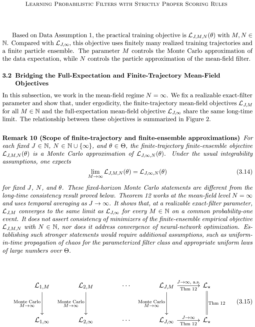
Under a realizability assumption, the population objective based on strictly proper scoring rules is minimized by the true Bayesian filtering distribution. The finite-ensemble empirical objective used in training is derived and related to the population objective via a mean-field consistency argument.
What carries the argument
The permutation-invariant transformer-based analysis map trained to minimize the energy score on synthetic state-observation trajectories.
If this is right
- The learned filter approximates nonlinear, non-Gaussian, and multi-modal posteriors from forecast ensembles and observations.
- Learning a correction to the ensemble Kalman filter is effective for problems close to Gaussian.
- An end-to-end learned map without the ensemble Kalman filter inductive bias performs better on highly non-Gaussian problems.
Where Pith is reading between the lines
- The same training procedure could be applied with other strictly proper scoring rules to emphasize different aspects of distributional accuracy.
- The approach may allow online filtering in systems where the true posterior cannot be computed analytically but synthetic trajectories are cheap to generate.
- Replacing the transformer with other permutation-invariant architectures might trade off expressivity against computational cost while preserving the optimality guarantee under realizability.
Load-bearing premise
The true Bayesian filtering distribution belongs to the hypothesis class of the chosen permutation-invariant transformer-based analysis map.
What would settle it
Train the model on a dynamical system whose exact filtering distribution is known to be representable by the transformer architecture, then check whether the output analysis ensembles match samples drawn from the true posterior on independent trajectories.
Figures


read the original abstract
Bayesian filtering of partially and noisily observed dynamical systems seeks to infer the evolving conditional distribution of the state of a dynamical system, given observations, in an online fashion. This Bayesian filtering distribution is the natural object for uncertainty quantification, but it is rarely available as a supervised learning target. However, one can often use the forecast model to generate synthetic system trajectories, along with synthetic observations. We introduce the proper scoring ensemble filter (PSEF), an ensemble data assimilation method based on training an analysis map to approximate the filtering distribution using only synthetic state--observation trajectories. The analysis step is represented as a permutation-invariant, transformer-based map that takes as input a forecast ensemble and observations, producing an analysis ensemble. Training is based on strictly proper scoring rules -- with the energy score used in our implementation -- so that probabilistic accuracy is rewarded over the whole probability distribution. We prove that, under a realizability assumption, the population objective is minimized by the true Bayesian filtering distribution. We also derive the finite-ensemble empirical objective used in training and relate its single state--observation trajectory form to the population objective, using a mean-field consistency argument. Numerical experiments show that the learned filter accurately approximates challenging filtering distributions, including nonlinear, non-Gaussian, and multi-modal posteriors, and achieves stronger performance in data assimilation tasks than classical methods or learning-based methods with mean-squared-error objectives. For close-to-Gaussian problems, learning a correction to the EnKF is the best approach, while for highly non-Gaussian problems an end-to-end approach that discards this inductive bias is superior.
Editorial analysis
A structured set of objections, weighed in public.
Referee Report
Summary. The paper introduces the Proper Scoring Ensemble Filter (PSEF), an ensemble data assimilation method that represents the analysis step as a permutation-invariant transformer-based map from forecast ensemble and observations to analysis ensemble. The map is trained on synthetic state-observation trajectories using the energy score (a strictly proper scoring rule) as the objective. The central theoretical result is a proof that, under a realizability assumption, the population objective is minimized exactly by the true Bayesian filtering distribution; a mean-field consistency argument is used to relate the single-trajectory empirical objective to the population objective. Experiments demonstrate accurate approximation of nonlinear, non-Gaussian, and multi-modal posteriors and superior data-assimilation performance relative to classical filters and MSE-trained baselines, with an end-to-end approach preferred for highly non-Gaussian cases.
Significance. If the realizability-based guarantee and mean-field derivation hold, the work supplies a principled, score-driven route to learning full probabilistic filters without direct posterior supervision. The explicit use of strict propriety (energy score) and the accompanying proof constitute a clear technical strength, as does the mean-field consistency argument that justifies the practical training objective. The empirical distinction between near-Gaussian and strongly non-Gaussian regimes supplies useful guidance for method selection in data assimilation.
minor comments (4)
- [§4.1, Eq. (8)] §4.1, Eq. (8): the finite-ensemble empirical objective is stated without an explicit statement of the Monte-Carlo estimator variance; adding a short remark on the number of synthetic trajectories required for stable gradients would improve reproducibility.
- [Figure 4] Figure 4: the multi-modal posterior visualization would benefit from an additional panel showing the energy-score calibration curve to make the claimed superiority over MSE objectives visually quantitative.
- [§5.3] §5.3: the statement that 'learning a correction to the EnKF is the best approach' for close-to-Gaussian problems is supported by the reported RMSE values, but the precise form of the learned correction (additive or multiplicative) is not specified; a one-sentence clarification would remove ambiguity.
- [References] References: the citation list omits the original energy-score paper (Gneiting & Raftery, 2007) despite using the score as the central training objective; adding it would strengthen the theoretical grounding.
Simulated Author's Rebuttal
We thank the referee for their positive summary of the manuscript, recognition of the theoretical contributions (realizability guarantee and mean-field argument), and recommendation for minor revision. No specific major comments were raised in the report.
Circularity Check
No significant circularity identified
full rationale
The central claim is a proof that the population objective (expected strictly proper score) is minimized by the true Bayesian filter under an explicit realizability assumption. This follows directly from the known definition of strict propriety for the energy score (an external fact, not constructed in the paper). The mean-field consistency relating empirical to population objective is a standard large-ensemble limit argument. No self-definitional reductions, fitted inputs renamed as predictions, or load-bearing self-citation chains appear; the derivation is self-contained against external benchmarks of proper scoring rules.
Axiom & Free-Parameter Ledger
axioms (1)
- domain assumption Realizability assumption: the true Bayesian filtering distribution lies in the hypothesis class of the transformer-based analysis map.
Reference graph
Works this paper leans on
-
[1]
Thomas Bengtsson, Peter Bickel, and Bo Li
doi: 10.1016/j.jcp.2025.114550. Thomas Bengtsson, Peter Bickel, and Bo Li. Curse-of-dimensionality revisited: Collapse of the particle filter in very large scale systems. InProbability and statistics: Essays in honor of David A. Freedman, volume 2, pages 316–335. Institute of Mathematical Statistics, 2008. Craig H Bishop, Brian J Etherton, and Sharanya J ...
-
[2]
Pierre Del Moral, Arnaud Doucet, and Ajay Jasra
IEEE, 2011. Pierre Del Moral, Arnaud Doucet, and Ajay Jasra. Sequential Monte Carlo samplers. Journal of the Royal Statistical Society Series B: Statistical Methodology, 68(3):411–436, 2006. Arnaud Doucet, Nando De Freitas, and Neil Gordon. An introduction to sequential Monte Carlo methods. InSequential Monte Carlo Methods in Practice, pages 3–14. Springe...
-
[3]
ISSN 1469-8080. doi: 10.1002/met.1409. Gregory Gaspari and Stephen E. Cohn. Construction of correlation functions in two and three dimensions.Quarterly Journal of the Royal Meteorological Society, 125(554):723– 757, 1999. doi: https://doi.org/10.1002/qj.49712555417. Borjan Geshkovski, Cyril Letrouit, Yury Polyanskiy, and Philippe Rigollet. The emergence o...
-
[4]
Peter L Houtekamer and Fuqing Zhang
doi: 10.1109/CDC.1994.410863. Peter L Houtekamer and Fuqing Zhang. Review of the ensemble Kalman filter for atmo- spheric data assimilation.Monthly Weather Review, 144(12):4489–4532, 2016. Guannan Hu, Sarah L. Dance, Ross N. Bannister, Hristo G. Chipilski, Oliver Guillet, Bruce Macpherson, Martin Weissmann, and Nusrat Yussouf. Progress, challenges, and fu...
-
[5]
ISSN 1942-2466. doi: 10.1029/2024MS004417. Manzil Zaheer, Satwik Kottur, Siamak Ravanbakhsh, Barnabas Poczos, Russ R Salakhut- dinov, and Alexander J Smola. Deep sets.Advances in Neural Information Processing Systems, 30, 2017. Xu-Hui Zhou, Zhuo-Ran Liu, and Heng Xiao. BI-EqNO: Generalized Approximate Bayesian Inference with an Equivariant Neural Operator...
-
[6]
For encoder blocks we useℓ= 1,
In the subscript (k, ℓ) of the self-attention blocksT s k,ℓ in (A.12), the indexk∈ {e, d} indicates whether the block belongs to the encoder (k=e) or the decoder (k=d). For encoder blocks we useℓ= 1, . . . , N e, and for decoder blocks we useℓ= 1 + Ne, . . . , Ne +N d
-
[7]
The cross-attention blockT c links encoder and decoder. Its first argumentp Ns ∈ P(R du) is an empirical measure supported onN s learnable points inR du, whereN s is a fixed hyperparameter that determines the size of the output feature matrix
-
[8]
57 Bach, Baptista, Br ¨ocker, Chen, and Stuart Appendix B
The trainable parameters consist of all parameters in the transformer blocks together with theN s learnable support points definingp Ns. 57 Bach, Baptista, Br ¨ocker, Chen, and Stuart Appendix B. Auxiliary Results To contextualize the lemmas presented in this section, we briefly recall the augmented state space formulation introduced in the main text. Not...
-
[9]
Here we sketch a methodology for establish- ing ergodicity of the resulting process, drawing on the approach described in Meyn and Tweedie (2012); Hairer (2021). This approach combines an assumed Lyapunov structure induced by the deterministic part of the dynamics, with a probabilistic analysis confined to a compact subset of phase space, using the contro...
2012
-
[10]
small sets
We denote byP q the probability law of the entire state trajectory (the probability measure on the path) initialized withv † 0 ∼q, i.e. Pq := Law {v† j }j∈Z+ |v † 0 ∼q ∈ P (Rdv)Z+ .(B.20) If the initial state is a deterministic point, i.e.,q=δ v† 0 , we writeP v† 0 . The corresponding expectation operator over these paths is denoted byE Pq. RecallPfrom (2...
2004
-
[11]
The resulting processes bZj = (bqj,bUj), bZ′ j = (bq′ j,bU ′ j) (B.42) form a valid coupling of the augmented processes with lawsP µ,Ω andP µ′,Ω
=µ ′.(B.40) Then define bqj+1 =F(bqj,byj+1),bq ′ j+1 =F(bq′ j,by′ j+1).(B.41) 65 Bach, Baptista, Br ¨ocker, Chen, and Stuart whereFis the map defined in Equation (B.27) which iterates the approximate filter. The resulting processes bZj = (bqj,bUj), bZ′ j = (bq′ j,bU ′ j) (B.42) form a valid coupling of the augmented processes with lawsP µ,Ω andP µ′,Ω. Eva...
2002
-
[12]
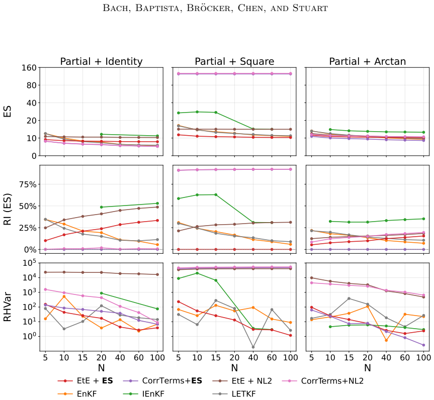
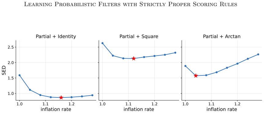
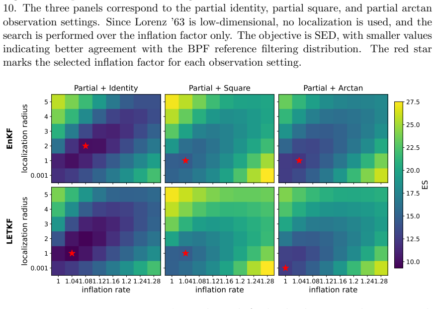
Since Lorenz ’63 is low-dimensional, no localization is used, and the search is performed over the inflation factor only
The three panels correspond to the partial identity, partial square, and partial arctan observation settings. Since Lorenz ’63 is low-dimensional, no localization is used, and the search is performed over the inflation factor only. The objective is SED, with smaller values indicating better agreement with the BPF reference filtering distribution. The red ...
1999
discussion (0)
Sign in with ORCID, Apple, or X to comment. Anyone can read and Pith papers without signing in.