Low-Luminosity Type IIP Supernovae from the Zwicky Transient Facility Census of the Local Universe. III: Hunting for electron-capture supernovae using nebular spectroscopy
Pith reviewed 2026-05-20 08:11 UTC · model grok-4.3
The pith
Nebular spectra of low-luminosity Type IIP supernovae set an upper limit on the electron-capture supernova rate.
A machine-rendered reading of the paper's core claim, the machinery that carries it, and where it could break.
Core claim
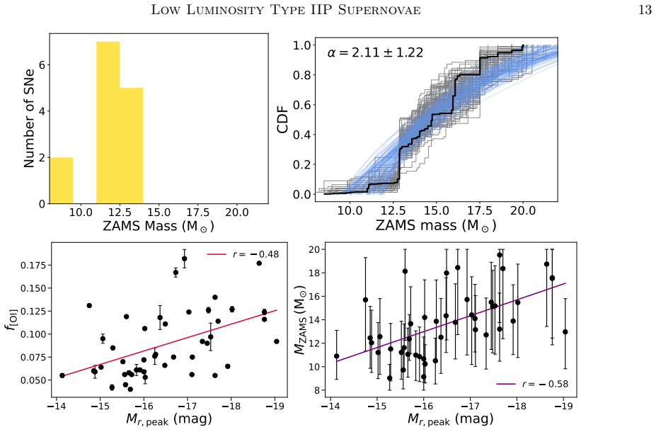
Combining the ZTF sample with literature data, the paper shows that low-luminosity Type IIP supernovae rarely exhibit the extremely narrow nebular hydrogen lines predicted for electron-capture supernovae from the lowest-mass core collapses, allowing an upper limit on the ECSN rate of ≲ (5–8)×10² Gpc^{-3} yr^{-1} and a progenitor mass window ΔM_sAGB ≲ 0.02–0.06 M_⊙ if they arise predominantly through the LLIIP channel.
What carries the argument
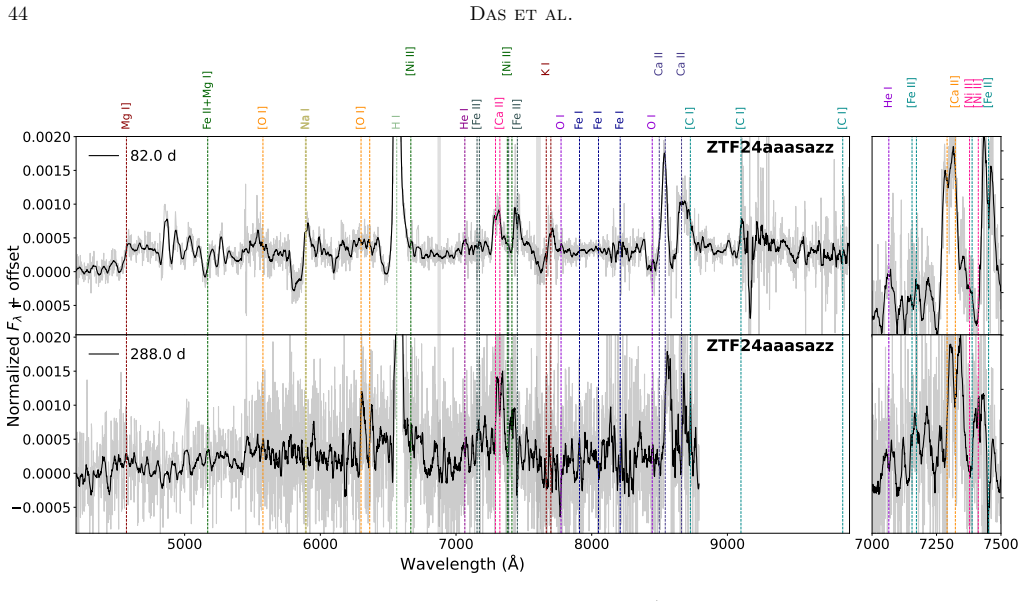
The ECSN score, which identifies candidates by the absence of He- and O-shell emission lines in nebular spectra, together with the full width at half maximum of the H I λ6563 line as a measure of explosion energy.
If this is right
- Low-luminosity Type IIP supernovae occupy the low-energy end of the core-collapse supernova population.
- The lack of correlation between hydrogen line width and plateau duration indicates that envelope and core properties are decoupled.
- Events with the extremely low energies predicted for ~9 solar mass progenitors are intrinsically rare.
- An IMF slope of 2.1±1.2 is inferred for the progenitors of Type II supernovae.
Where Pith is reading between the lines
- Current theoretical models for the nebular line widths in the weakest ECSNe may require refinement if no events match the predictions.
- Electron-capture supernovae could occur through channels other than low-luminosity Type IIP events.
- The narrow mass window suggests that only a small fraction of super-asymptotic giant branch stars successfully explode as electron-capture supernovae rather than forming white dwarfs.
Load-bearing premise
The assumption that the absence of extremely narrow nebular hydrogen lines in the candidate events rules out standard electron-capture supernova models depends on the accuracy of current theoretical predictions for line widths in the weakest explosions around 9 solar masses.
What would settle it
Detection of a low-luminosity Type IIP supernova that scores high on the ECSN criteria and also displays the extremely narrow H I λ6563 line widths predicted by the weakest explosion models would support a higher rate or confirm the model predictions.
Figures


read the original abstract
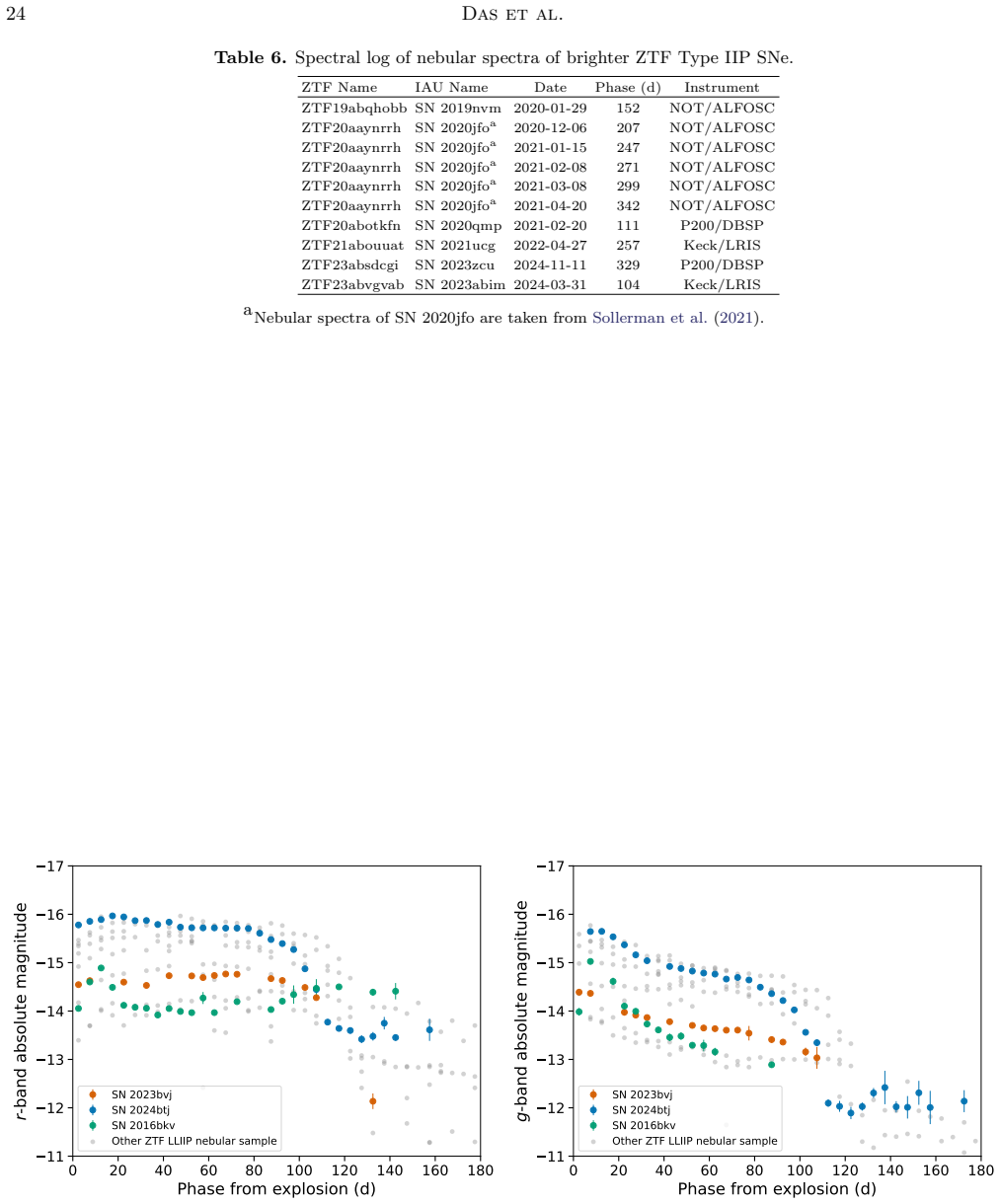
Electron-capture supernovae (ECSNe) may arise from ONeMg-core collapse in super-asymptotic giant branch (sAGB) stars near the low-mass core-collapse limit ($\approx\!8$--$10$\,\Msun). At early times, models predict that ECSNe resemble low-mass red supergiant iron-core-collapse SNe (FeCCSNe), making the two channels difficult to distinguish. Nebular spectroscopy, however, can reveal differences in ejecta composition. We present a systematic sample of nebular spectra of 19 low-luminosity Type IIP (LLIIP) SNe from the ZTF CLU survey, obtained 115$-$450\,d after explosion. Their low velocities expose narrow lines blended in brighter SNe, which we identify and model to constrain progenitor properties. We find a strong correlation between the FWHM of H\,\textsc{i}\,$\lambda$6563 and peak luminosity, showing that LLIIP SNe occupy the low-energy end of the core-collapse population, but no correlation with plateau duration, suggesting that envelope and core properties are not tightly linked. Only one SN reaches the extremely low H\,\textsc{i}\,$\lambda$6563 widths predicted for the weakest $\sim$9\,M$_\odot$ explosion models, implying that such low-energy events are intrinsically rare. Combining our sample with 118 literature nebular spectra of Type II SNe, we infer an IMF slope of $2.1\pm1.2$. We also introduce an `ECSN score'' based on the absence of He- and O-shell emission lines, and identify two plausible ECSN candidates, SN~2023bvj and SN~2024btj. However, neither shows the extremely narrow nebular lines predicted by current ECSN models. If ECSNe arise predominantly through the LLIIP channel, we infer an upper limit on the ECSN rate of $\lesssim (5$--$8)\times10^{2}\,\mathrm{Gpc^{-3}\,yr^{-1}}$, corresponding to a narrow sAGB progenitor mass window of $\Delta M_{\rm sAGB} \lesssim 0.02$--$0.06\,\mathrm{M_\odot}$.
Editorial analysis
A structured set of objections, weighed in public.
Referee Report
Summary. The manuscript analyzes nebular spectra of 19 low-luminosity Type IIP supernovae from the ZTF CLU survey obtained 115-450 days post-explosion. It reports a strong correlation between H I λ6563 FWHM and peak luminosity (but none with plateau duration), introduces an empirically defined 'ECSN score' based on the absence of He- and O-shell emission lines, identifies two plausible ECSN candidates (SN 2023bvj and SN 2024btj), and combines the sample with 118 literature Type II spectra to infer an IMF slope of 2.1±1.2. Assuming ECSNe arise predominantly via the LLIIP channel, it derives an upper limit on the ECSN rate of ≲(5–8)×10² Gpc^{-3} yr^{-1}, implying a narrow sAGB progenitor mass window of ΔM_sAGB ≲0.02–0.06 M_⊙.
Significance. If the central claims hold, the work supplies a systematic observational sample at the faint end of the core-collapse population and places quantitative limits on the ECSN channel that are directly relevant to stellar evolution models near the 8–10 M_⊙ boundary. The reported FWHM–luminosity correlation and the introduction of an ECSN score constitute useful empirical advances, though the rate upper limit rests on theoretical line-width predictions.
major comments (1)
- [Abstract and rate-derivation section] Abstract and the section deriving the ECSN rate upper limit: the inference that the absence of extremely narrow H I λ6563 lines in the two high-ECSN-score candidates (SN 2023bvj and SN 2024btj) rules out standard ~9 M_⊙ ONeMg-core models (and thereby yields the ≲(5–8)×10² Gpc^{-3} yr^{-1} limit) depends on the robustness of current theoretical FWHM predictions; no sensitivity analysis to variations in explosion energy, 56Ni mixing, or residual H-envelope mass is presented, which is load-bearing for the rate and mass-window conclusions.
minor comments (2)
- [Methods] Provide the precise numerical definition and weighting of the 'ECSN score' (including which lines are required to be absent) so that the classification of the two candidates can be reproduced from the spectra.
- [Results] Clarify whether the IMF slope of 2.1±1.2 is derived solely from the combined sample or incorporates additional assumptions about the LLIIP fraction; state the exact fitting procedure and any selection-function corrections applied to the heterogeneous literature data.
Simulated Author's Rebuttal
We thank the referee for their constructive review and for highlighting the importance of assessing the robustness of the theoretical line-width predictions underlying our ECSN rate limit. We address the major comment below and outline planned revisions.
read point-by-point responses
-
Referee: [Abstract and rate-derivation section] Abstract and the section deriving the ECSN rate upper limit: the inference that the absence of extremely narrow H I λ6563 lines in the two high-ECSN-score candidates (SN 2023bvj and SN 2024btj) rules out standard ~9 M_⊙ ONeMg-core models (and thereby yields the ≲(5–8)×10² Gpc^{-3} yr^{-1} limit) depends on the robustness of current theoretical FWHM predictions; no sensitivity analysis to variations in explosion energy, 56Ni mixing, or residual H-envelope mass is presented, which is load-bearing for the rate and mass-window conclusions.
Authors: We agree that the rate upper limit and implied sAGB mass window rest on the assumption that current ECSN models reliably predict extremely narrow H I λ6563 lines for standard ~9 M_⊙ ONeMg-core progenitors. The manuscript cites specific model predictions (e.g., from the literature on low-energy ECSN explosions) showing FWHM values well below those observed in our sample, including the two high-ECSN-score candidates. While a comprehensive sensitivity study varying explosion energy, 56Ni mixing, and residual H-envelope mass was not included, the available models indicate that even moderate increases in these parameters do not produce the observed line widths without violating other constraints (such as the low luminosities and plateau properties). We will revise the rate-derivation section and abstract to explicitly discuss these model dependencies, add qualitative sensitivity considerations drawn from existing ECSN and low-energy FeCCSN simulations, and qualify the upper limit as model-dependent. This will make the load-bearing assumptions transparent without altering the core observational result that no object in the sample matches the narrowest predicted lines. revision: yes
Circularity Check
No significant circularity; derivation uses independent observational spectra and external model comparisons
full rationale
The paper's central inference—an upper limit on the ECSN rate conditional on the LLIIP channel—rests on new ZTF nebular spectra of 19 LLIIP events, a measured FWHM-luminosity correlation, an empirically defined ECSN score from missing He/O lines, and comparison to cited theoretical predictions for line widths in ~9 M⊙ models. No step reduces a fitted parameter to a renamed prediction, defines a quantity in terms of itself, or relies on a load-bearing self-citation whose validity is internal to the present work. The IMF slope and rate limit are derived from the combined sample and model assumptions that remain falsifiable against external benchmarks.
Axiom & Free-Parameter Ledger
free parameters (1)
- IMF slope =
2.1 ± 1.2
axioms (1)
- domain assumption Nebular spectra at 115-450 days reveal composition differences that distinguish ECSNe from iron-core-collapse SNe
invented entities (1)
-
ECSN score
no independent evidence
Lean theorems connected to this paper
-
IndisputableMonolith/Foundation/RealityFromDistinction.leanreality_from_one_distinction unclear?
unclearRelation between the paper passage and the cited Recognition theorem.
We find a strong correlation between the FWHM of H I λ6563 and peak luminosity... Only one SN reaches the extremely low H I λ6563 widths predicted for the weakest ∼9 M⊙ explosion models... If ECSNe arise predominantly through the LLIIP channel, we infer an upper limit on the ECSN rate of ≲(5–8)×10² Gpc⁻³ yr⁻¹, corresponding to a narrow sAGB progenitor mass window of ΔM_sAGB ≲0.02–0.06 M⊙.
What do these tags mean?
- matches
- The paper's claim is directly supported by a theorem in the formal canon.
- supports
- The theorem supports part of the paper's argument, but the paper may add assumptions or extra steps.
- extends
- The paper goes beyond the formal theorem; the theorem is a base layer rather than the whole result.
- uses
- The paper appears to rely on the theorem as machinery.
- contradicts
- The paper's claim conflicts with a theorem or certificate in the canon.
- unclear
- Pith found a possible connection, but the passage is too broad, indirect, or ambiguous to say the theorem truly supports the claim.
Reference graph
Works this paper leans on
-
[1]
Adams, S. M., Kochanek, C. S., Prieto, J. L., et al. 2016, MNRAS, 460, 1645, doi: 10.1093/mnras/stw1059
-
[2]
2023, MNRAS, 519, 248, doi: 10.1093/mnras/stac3234
Ailawadhi, B., Dastidar, R., Misra, K., et al. 2023, MNRAS, 519, 248, doi: 10.1093/mnras/stac3234
-
[3]
Anderson, J. P., Dessart, L., Gutierrez, C. P., et al. 2014, MNRAS, 441, 671, doi: 10.1093/mnras/stu610
-
[4]
P., Dessart, L., Guti´ errez, C
Anderson, J. P., Dessart, L., Guti´ errez, C. P., et al. 2018, Nature Astronomy, 2, 574, doi: 10.1038/s41550-018-0458-4
-
[5]
Andrews, J. E., Sugerman, B. E. K., Clayton, G. C., et al. 2011, ApJ, 731, 47, doi: 10.1088/0004-637X/731/1/47
-
[6]
E., Pearson, J., Hosseinzadeh, G., et al
Andrews, J. E., Pearson, J., Hosseinzadeh, G., et al. 2024, ApJ, 965, 85, doi: 10.3847/1538-4357/ad2a49 Astropy Collaboration, Robitaille, T. P., Tollerud, E. J., et al. 2013, A&A, 558, A33, doi: 10.1051/0004-6361/201322068
-
[7]
2024, MNRAS, 533, 1251, doi: 10.1093/mnras/stae1811
Barmentloo, S., Jerkstrand, A., Iwamoto, K., et al. 2024, MNRAS, 533, 1251, doi: 10.1093/mnras/stae1811
-
[8]
Bellm, E. C., & Sesar, B. 2016, pyraf-dbsp: Reduction pipeline for the Palomar Double Beam Spectrograph, Astrophysics Source Code Library. http://ascl.net/1602.002
work page 2016
-
[9]
Bellm, E. C., Kulkarni, S. R., Graham, M. J., et al. 2019, PASP, 131, 018002, doi: 10.1088/1538-3873/aaecbe
-
[10]
Benetti, S., Turatto, M., Balberg, S., et al. 2001, MNRAS, 322, 361, doi: 10.1046/j.1365-8711.2001.04122.x
-
[11]
S., Milisavljevic, D., Margutti, R., et al
Black, C. S., Milisavljevic, D., Margutti, R., et al. 2017, ApJ, 848, 5, doi: 10.3847/1538-4357/aa8999
-
[12]
Blanton, E. L., Schmidt, B. P., Kirshner, R. P., et al. 1995, AJ, 110, 2868, doi: 10.1086/117735
-
[13]
2013, MNRAS, 433, 1871, doi: 10.1093/mnras/stt864 Low Luminosity Type IIP Supernovae19
Bose, S., Kumar, B., Sutaria, F., et al. 2013, MNRAS, 433, 1871, doi: 10.1093/mnras/stt864 Low Luminosity Type IIP Supernovae19
-
[14]
2015, ApJ, 806, 160, doi: 10.1088/0004-637X/806/2/160
Bose, S., Sutaria, F., Kumar, B., et al. 2015, ApJ, 806, 160, doi: 10.1088/0004-637X/806/2/160
-
[15]
A., Valenti, S., Horesh, A., et al
Bostroem, K. A., Valenti, S., Horesh, A., et al. 2019, MNRAS, 485, 5120, doi: 10.1093/mnras/stz570
-
[16]
Bostroem, K. A., Dessart, L., Hillier, D. J., et al. 2023, ApJL, 953, L18, doi: 10.3847/2041-8213/ace31c
-
[17]
2009, MNRAS, 395, 472, doi: 10.1111/j.1365-2966.2009.14539.x
Botticella, M. T., Pastorello, A., Smartt, S. J., et al. 2009, MNRAS, 398, 1041, doi: 10.1111/j.1365-2966.2009.15082.x
-
[18]
2007, in American Institute of Physics Conference Series, Vol
Bufano, F., Benetti, S., Turatto, M., et al. 2007, in American Institute of Physics Conference Series, Vol. 924, The Multicolored Landscape of Compact Objects and Their Explosive Origins, ed. T. di Salvo, G. L. Israel, L. Piersant, L. Burderi, G. Matt, A. Tornambe, & M. T. Menna (AIP), 271–276, doi: 10.1063/1.2774869
-
[19]
2019, MNRAS, 485, 3153, doi: 10.1093/mnras/stz543
Burrows, A., Radice, D., & Vartanyan, D. 2019, MNRAS, 485, 3153, doi: 10.1093/mnras/stz543
-
[20]
2024, ApJL, 964, L16, doi: 10.3847/2041-8213/ad319e
Burrows, A., Wang, T., & Vartanyan, D. 2024, ApJL, 964, L16, doi: 10.3847/2041-8213/ad319e
-
[21]
Byrne, C. M., Eldridge, J. J., & Stanway, E. R. 2025, MNRAS, 537, 2433, doi: 10.1093/mnras/staf178
-
[22]
2021, arXiv e-prints, arXiv:2109.12943, doi: 10.48550/arXiv.2109.12943
Callis, E., Fraser, M., Pastorello, A., et al. 2021, arXiv e-prints, arXiv:2109.12943, doi: 10.48550/arXiv.2109.12943
-
[23]
Chornock, R., Filippenko, A. V., Li, W., & Silverman, J. M. 2010, ApJ, 713, 1363, doi: 10.1088/0004-637X/713/2/1363
-
[24]
Clocchiatti, A., Benetti, S., Wheeler, J. C., et al. 1996, AJ, 111, 1286, doi: 10.1086/117874
-
[25]
Coughlin, M. W., Bloom, J. S., Nir, G., et al. 2023, ApJS, 267, 31, doi: 10.3847/1538-4365/acdee1
-
[26]
Das, K. K., Kasliwal, M. M., Fremling, C., et al. 2025, PASP, 137, 044203, doi: 10.1088/1538-3873/adcaeb
-
[27]
Das, K. K., Kasliwal, M. M., Sollerman, J., et al. 2026, PASP, 138, 024204, doi: 10.1088/1538-3873/ae33f5
-
[28]
2025, arXiv e-prints, arXiv:2501.01530
Dastidar, R., Misra, K., Valenti, S., et al. 2025, arXiv e-prints, arXiv:2501.01530. https://arxiv.org/abs/2501.01530
-
[29]
De, K., Kasliwal, M. M., Tzanidakis, A., et al. 2020, ApJ, 905, 58, doi: 10.3847/1538-4357/abb45c de Jaeger, T., Zheng, W., Stahl, B. E., et al. 2019, MNRAS, 490, 2799, doi: 10.1093/mnras/stz2714
-
[30]
Dekany, R., Smith, R. M., Riddle, R., et al. 2020, PASP, 132, 038001, doi: 10.1088/1538-3873/ab4ca2
-
[31]
Dessart, L., & Hillier, D. J. 2020, A&A, 642, A33, doi: 10.1051/0004-6361/202038148
-
[32]
Janka, H. T. 2021a, A&A, 656, A61, doi: 10.1051/0004-6361/202141927 —. 2021b, A&A, 652, A64, doi: 10.1051/0004-6361/202140839
-
[33]
2025, arXiv e-prints, arXiv:2507.05803, doi: 10.48550/arXiv.2507.05803
Dessart, L., Kotak, R., Jacobson-Galan, W., et al. 2025, arXiv e-prints, arXiv:2507.05803, doi: 10.48550/arXiv.2507.05803
-
[34]
Lau, H. H. B. 2015, MNRAS, 446, 2599, doi: 10.1093/mnras/stu2180
-
[35]
Dong, Y., Valenti, S., Bostroem, K. A., et al. 2021, ApJ, 906, 56, doi: 10.3847/1538-4357/abc417
-
[36]
Drake, A. J., Djorgovski, S. G., Graham, M. J., et al. 2012, Central Bureau Electronic Telegrams, 3118, 1
work page 2012
-
[37]
Duev, D. A., Mahabal, A., Masci, F. J., et al. 2019, arXiv e-prints. https://arxiv.org/abs/1907.11259
-
[38]
Eldridge, J. J., Stanway, E. R., Xiao, L., et al. 2017, PASA, 34, e058, doi: 10.1017/pasa.2017.51
work page internal anchor Pith review doi:10.1017/pasa.2017.51 2017
-
[39]
Elias-Rosa, N., Van Dyk, S. D., Li, W., et al. 2009, ApJ, 706, 1174, doi: 10.1088/0004-637X/706/2/1174
-
[40]
Elmhamdi, A., Danziger, I. J., Chugai, N., et al. 2003, MNRAS, 338, 939, doi: 10.1046/j.1365-8711.2003.06150.x
-
[41]
Fang, Q., Moriya, T. J., & Maeda, K. 2025, ApJ, 986, 39, doi: 10.3847/1538-4357/adceae
-
[42]
Faran, T., Poznanski, D., Filippenko, A. V., et al. 2014, MNRAS, 442, 844, doi: 10.1093/mnras/stu955
-
[43]
Andrews, J. E. 2024, A&A, 687, L20, doi: 10.1051/0004-6361/202450440
-
[44]
Fransson, C., & Chevalier, R. A. 1989, ApJ, 343, 323, doi: 10.1086/167707
-
[45]
Fraser, M., Ergon, M., Eldridge, J. J., et al. 2011, MNRAS, 417, 1417, doi: 10.1111/j.1365-2966.2011.19370.x G´ omez, G., & L´ opez, R. 2000, AJ, 120, 367, doi: 10.1086/301419
-
[46]
Graham, M. J., Kulkarni, S. R., Bellm, E. C., et al. 2019, PASP, 131, 078001, doi: 10.1088/1538-3873/ab006c
-
[47]
Guillochon, J., Parrent, J., Kelley, L. Z., & Margutti, R. 2017, ApJ, 835, 64, doi: 10.3847/1538-4357/835/1/64
-
[48]
Chakradhari, N. K. 2008, Bulletin of the Astronomical Society of India, 36, 79 Guti´ errez, C. P., Anderson, J. P., Hamuy, M., et al. 2017, ApJ, 850, 89, doi: 10.3847/1538-4357/aa8f52 Guti´ errez, C. P., Pastorello, A., Jerkstrand, A., et al. 2020, MNRAS, 499, 974, doi: 10.1093/mnras/staa2763 Guti´ errez, J., Canal, R., & Garc´ ıa-Berro, E. 2005, A&A, 435...
-
[49]
Hendry, M. A., Smartt, S. J., Maund, J. R., et al. 2005, MNRAS, 359, 906, doi: 10.1111/j.1365-2966.2005.08928.x 20Das et al
-
[50]
Hendry, M. A., Smartt, S. J., Crockett, R. M., et al. 2006, MNRAS, 369, 1303, doi: 10.1111/j.1365-2966.2006.10374.x
-
[51]
Hiramatsu, D., Howell, D. A., Van Dyk, S. D., et al. 2021, Nature Astronomy, 5, 903, doi: 10.1038/s41550-021-01384-2
-
[52]
2018, ApJ, 861, 63, doi: 10.3847/1538-4357/aac5f6
Hosseinzadeh, G., Valenti, S., McCully, C., et al. 2018, ApJ, 861, 63, doi: 10.3847/1538-4357/aac5f6
-
[53]
2016, ApJ, 832, 139, doi: 10.3847/0004-637X/832/2/139
Huang, F., Wang, X., Zampieri, L., et al. 2016, ApJ, 832, 139, doi: 10.3847/0004-637X/832/2/139
-
[54]
2018, MNRAS, 475, 3959, doi: 10.1093/mnras/sty066
Huang, F., Wang, X.-F., Hosseinzadeh, G., et al. 2018, MNRAS, 475, 3959, doi: 10.1093/mnras/sty066
-
[55]
Hunter, J. D. 2007, Computing In Science & Engineering, 9, 90, doi: 10.1109/MCSE.2007.55
-
[56]
2013, A&A, 555, A142, doi: 10.1051/0004-6361/201220496
Inserra, C., Pastorello, A., Turatto, M., et al. 2013, A&A, 555, A142, doi: 10.1051/0004-6361/201220496
-
[57]
2012, Central Bureau Electronic Telegrams, 3338, 1 Jacobson-Gal´ an, W
Itagaki, K., Noguchi, T., Nakano, S., et al. 2012, Central Bureau Electronic Telegrams, 3338, 1 Jacobson-Gal´ an, W. V., Dessart, L., Davis, K. W., et al. 2025, ApJ, 992, 100, doi: 10.3847/1538-4357/adfa23 J¨ ager, Zolt´ an, J., Vink´ o, J., B´ ır´ o, B. I., et al. 2020, MNRAS, 496, 3725, doi: 10.1093/mnras/staa1743
-
[58]
Janka, H. T., M¨ uller, B., Kitaura, F. S., & Buras, R. 2008, A&A, 485, 199, doi: 10.1051/0004-6361:20079334
-
[59]
Jencson, J. E., Adams, S. M., Bond, H. E., et al. 2019, ApJL, 880, L20, doi: 10.3847/2041-8213/ab2c05
-
[60]
Jerkstrand, A., Ergon, M., Smartt, S. J., et al. 2015a, A&A, 573, A12, doi: 10.1051/0004-6361/201423983
-
[61]
Jerkstrand, A., Ertl, T., Janka, H. T., et al. 2018, MNRAS, 475, 277, doi: 10.1093/mnras/stx2877
-
[62]
2011, A&A, 530, A45, doi: 10.1051/0004-6361/201015937
Jerkstrand, A., Fransson, C., & Kozma, C. 2011, A&A, 530, A45, doi: 10.1051/0004-6361/201015937
-
[63]
2012, A&A, 546, A28, doi: 10.1051/0004-6361/201219528
Jerkstrand, A., Fransson, C., Maguire, K., et al. 2012, A&A, 546, A28, doi: 10.1051/0004-6361/201219528
-
[64]
Jerkstrand, A., Smartt, S. J., Fraser, M., et al. 2014a, MNRAS, 439, 3694, doi: 10.1093/mnras/stu221 —. 2014b, MNRAS, 439, 3694, doi: 10.1093/mnras/stu221
-
[65]
Jerkstrand, A., Smartt, S. J., Sollerman, J., et al. 2015b, MNRAS, 448, 2482, doi: 10.1093/mnras/stv087 —. 2015c, MNRAS, 448, 2482, doi: 10.1093/mnras/stv087
-
[66]
2013, ApJ, 772, 150, doi: 10.1088/0004-637X/772/2/150
Jones, S., Hirschi, R., Nomoto, K., et al. 2013, ApJ, 772, 150, doi: 10.1088/0004-637X/772/2/150
-
[67]
M., Cannella, C., Bagdasaryan, A., et al
Kasliwal, M. M., Cannella, C., Bagdasaryan, A., et al. 2019, PASP, 131, 038003, doi: 10.1088/1538-3873/aafbc2
-
[68]
M., Fremling, C., Yan, L., et al
Kasliwal, M. M., Fremling, C., Yan, L., et al. 2024, Transient Name Server AstroNote, 340, 1
work page 2024
-
[69]
Kilpatrick, C. D., Foley, R. J., Jacobson-Gal´ an, W. V., et al. 2023, ApJL, 952, L23, doi: 10.3847/2041-8213/ace4ca
-
[70]
Kitaura, F. S., Janka, H. T., & Hillebrandt, W. 2006, A&A, 450, 345, doi: 10.1051/0004-6361:20054703
-
[71]
2022, MNRAS, 514, 4173, doi: 10.1093/mnras/stac1518
Kozyreva, A., Janka, H.-T., Kresse, D., Taubenberger, S., & Baklanov, P. 2022, MNRAS, 514, 4173, doi: 10.1093/mnras/stac1518
-
[72]
Leonard, D. C., Filippenko, A. V., Ganeshalingam, M., et al. 2006, Nature, 440, 505, doi: 10.1038/nature04558
-
[73]
Li, W., Van Dyk, S. D., Filippenko, A. V., et al. 2006, ApJ, 641, 1060, doi: 10.1086/499916
-
[74]
Maguire, K., Jerkstrand, A., Smartt, S. J., et al. 2012, MNRAS, 420, 3451, doi: 10.1111/j.1365-2966.2011.20276.x
-
[75]
Masci, F. J., Laher, R. R., Rusholme, B., et al. 2019, PASP, 131, 018003, doi: 10.1088/1538-3873/aae8ac
work page internal anchor Pith review doi:10.1088/1538-3873/aae8ac 2019
-
[76]
Mattila, S., Smartt, S. J., Eldridge, J. J., et al. 2008, ApJL, 688, L91, doi: 10.1086/595587
-
[77]
Maund, J. R., Smartt, S. J., & Danziger, I. J. 2005, MNRAS, 364, L33, doi: 10.1111/j.1745-3933.2005.00100.x
-
[78]
Meza-Retamal, N., Dong, Y., Bostroem, K. A., et al. 2024, ApJ, 971, 141, doi: 10.3847/1538-4357/ad4d55
-
[79]
1980, PASJ, 32, 303 M¨ uller-Bravo, T
Miyaji, S., Nomoto, K., Yokoi, K., & Sugimoto, D. 1980, PASJ, 32, 303 M¨ uller-Bravo, T. E., Guti´ errez, C. P., Sullivan, M., et al. 2020, MNRAS, 497, 361, doi: 10.1093/mnras/staa1932
-
[80]
2024, MNRAS, 528, 4209, doi: 10.1093/mnras/stae170
Murai, Y., Tanaka, M., Kawabata, M., et al. 2024, MNRAS, 528, 4209, doi: 10.1093/mnras/stae170
discussion (0)
Sign in with ORCID, Apple, or X to comment. Anyone can read and Pith papers without signing in.