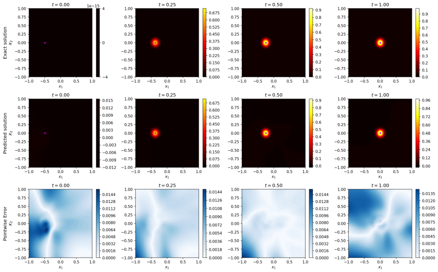
DAS-PINNs for high-dimensional partial differential equations: extending deep adaptive sampling to spacetime domains
Pith reviewed 2026-06-28 00:08 UTC · model grok-4.3
The pith
A normalizing flow learns the PDE residual distribution to generate adaptive collocation points across unified spacetime domains.
A machine-rendered reading of the paper's core claim, the machinery that carries it, and where it could break.
Core claim
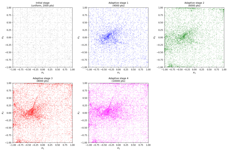
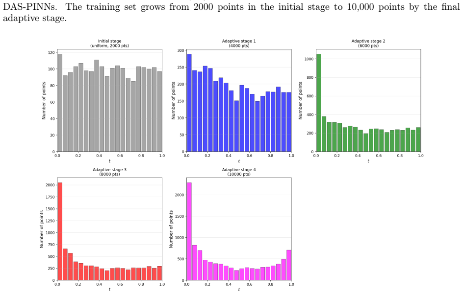
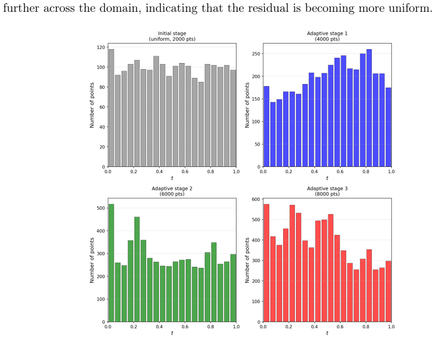
A normalising flow neural network model effectively learns the distribution induced by the PDE residual and generates new collocation points concentrated in regions where the solution is most difficult to learn. Unlike conventional adaptive strategies that require explicit time stepping or moving meshes, high-residual regions are automatically identified and tracked across both space and time, driven purely by the PDE residual distribution.
What carries the argument
Normalizing flow neural network that learns the distribution induced by the PDE residual to produce new collocation points
If this is right
- High-residual regions are tracked across space and time without explicit time marching or moving meshes.
- The method applies to problems with sharp and moving features in two spatial dimensions.
- Localized structures can be resolved in up to eight spatial dimensions.
- Uniform collocation sampling is replaced by residual-driven adaptive sampling in a single spacetime domain.
Where Pith is reading between the lines
- Fewer total collocation points may suffice for the same accuracy once sampling concentrates on difficult regions.
- The same residual-driven flow idea could be tested on other mesh-free PDE solvers beyond PINNs.
- Performance on problems whose residual distribution changes rapidly in time would reveal how often the flow must be retrained.
Load-bearing premise
The normalizing flow can learn the PDE residual distribution in the unified spacetime domain accurately enough to generate useful adaptive samples.
What would settle it
On a benchmark problem, the training error of the PINN remains the same or higher when collocation points are chosen by the flow compared with uniform sampling.
Figures


read the original abstract
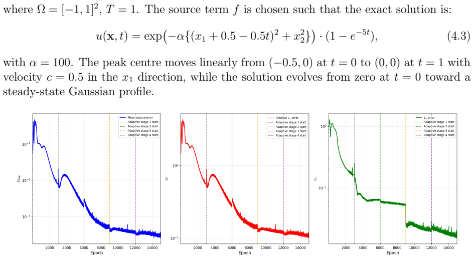
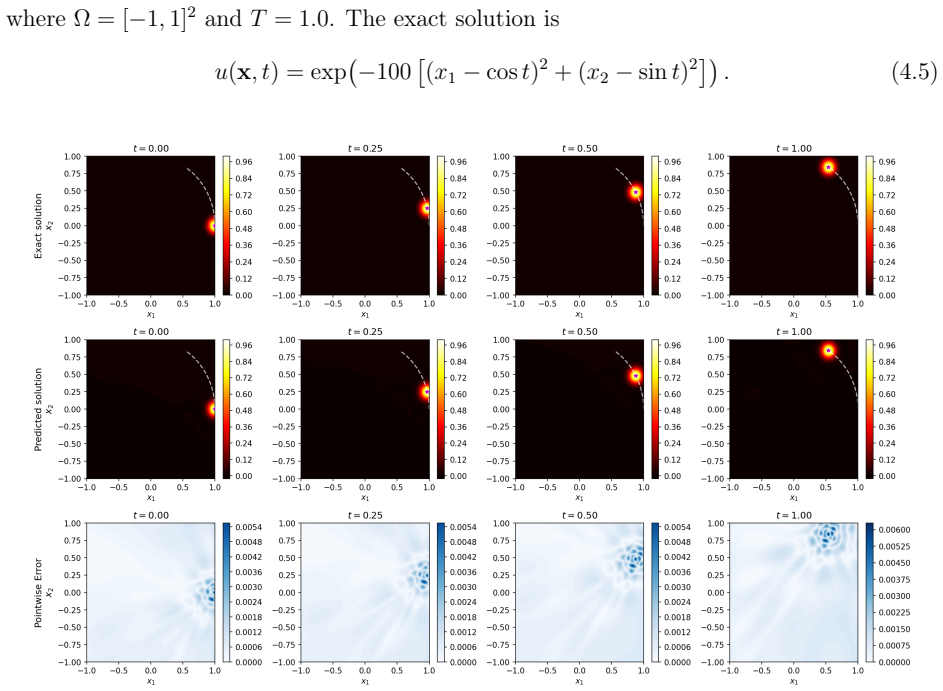
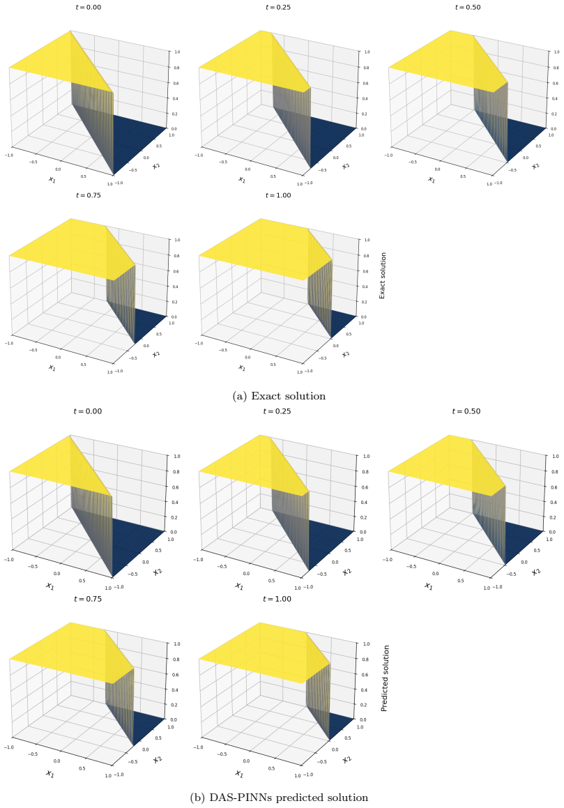
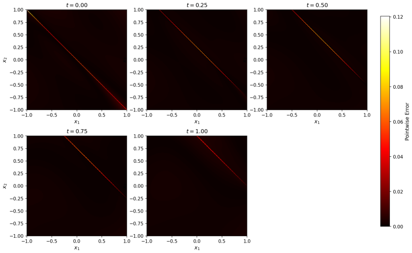
Time-dependent high-dimensional partial differential equations (PDEs) with spatially localised and dynamically evolving solutions pose a fundamental challenge for physics-informed neural networks (PINNs), as uniform collocation sampling becomes increasingly ineffective in high-dimensional spatiotemporal domains. In this work, a deep adaptive sampling framework for PINNs is extended to the time-dependent setting by treating space and time as a unified domain without any explicit time marching. A normalising flow neural network model effectively learns the distribution induced by the PDE residual and generates new collocation points concentrated in regions where the solution is most difficult to learn. Unlike conventional adaptive strategies that require explicit time stepping or moving meshes, high-residual regions are automatically identified and tracked across both space and time, driven purely by the PDE residual distribution. The effectiveness of the proposed strategy is assessed on a range of benchmark problems, from sharp and moving features in two spatial dimensions to localised structures in up to eight spatial dimensions.
Editorial analysis
A structured set of objections, weighed in public.
Referee Report
Summary. The paper claims to extend deep adaptive sampling (DAS) for physics-informed neural networks (PINNs) to time-dependent high-dimensional PDEs by treating the spacetime domain as unified (without explicit time marching or moving meshes). A normalizing flow is used to learn the distribution induced by the PDE residual and to generate adaptive collocation points concentrated in high-residual regions. Effectiveness is assessed via benchmarks involving sharp/moving features in 2D and localized structures up to 8 spatial dimensions plus time.
Significance. If the central claim holds, the work could advance adaptive collocation strategies for PINNs on evolutionary PDEs in high dimensions by automating residual-driven sampling over a single spacetime domain. The approach avoids conventional time-stepping requirements, which is a practical strength for problems with dynamically evolving localized features. No machine-checked proofs, parameter-free derivations, or open reproducible code are referenced.
major comments (2)
- [Abstract] Abstract: The assertion that the normalizing flow 'effectively learns' the residual distribution and produces useful adaptive samples lacks any referenced quantitative diagnostics (KL divergence, effective sample size, coverage of high-residual regions, or direct comparison to ground-truth residual histograms) for the 8D+time cases. This is load-bearing because downstream PINN accuracy improvements could result from increased total collocation points or optimizer choices rather than faithful approximation of the (potentially multimodal, non-stationary) residual distribution.
- [Numerical experiments] Numerical experiments section: No ablation studies or isolated metrics are supplied that separate the normalizing flow's density estimation quality from other implementation factors, leaving the weakest assumption (accurate learning of the residual distribution in unified spacetime without time marching) untested directly.
Simulated Author's Rebuttal
We thank the referee for their thoughtful review and constructive suggestions. We address each major comment below, providing clarifications and indicating where revisions will strengthen the manuscript.
read point-by-point responses
-
Referee: [Abstract] The assertion that the normalizing flow 'effectively learns' the residual distribution and produces useful adaptive samples lacks any referenced quantitative diagnostics (KL divergence, effective sample size, coverage of high-residual regions, or direct comparison to ground-truth residual histograms) for the 8D+time cases. This is load-bearing because downstream PINN accuracy improvements could result from increased total collocation points or optimizer choices rather than faithful approximation of the (potentially multimodal, non-stationary) residual distribution.
Authors: We acknowledge that the manuscript does not include explicit quantitative diagnostics such as KL divergence or direct histogram comparisons for the normalizing flow in the 8D+time cases. The effectiveness is instead shown indirectly through benchmark results demonstrating lower errors with adaptive sampling versus uniform sampling at fixed total collocation point counts. In high dimensions, direct ground-truth residual histograms are computationally intractable. We will add KL divergence, effective sample size, and coverage metrics for the 2D cases in the revised version; for higher dimensions the downstream performance on moving and localized features provides supporting evidence that the improvements stem from residual-driven adaptation rather than point count or optimizer alone. revision: partial
-
Referee: [Numerical experiments] No ablation studies or isolated metrics are supplied that separate the normalizing flow's density estimation quality from other implementation factors, leaving the weakest assumption (accurate learning of the residual distribution in unified spacetime without time marching) untested directly.
Authors: The current numerical section compares the complete DAS-PINNs method against uniform-sampling PINNs on problems with sharp moving features (2D) and localized structures (up to 8D+time), with the same total collocation budget. While this does not isolate the flow's density estimation in an ablation, the consistent gains on non-stationary problems support that the unified spacetime sampling tracks high-residual regions without explicit time marching. We agree dedicated ablations would strengthen the presentation and will add them for the lower-dimensional benchmarks in revision, including comparisons of learned versus uniform distributions. revision: yes
Circularity Check
No circularity: method effectiveness evaluated on external benchmarks
full rationale
The paper extends a normalizing-flow-based adaptive sampling procedure to spacetime PINN collocation by training the flow on the PDE residual and sampling from the learned density. This construction is not self-definitional because the claim that the resulting points improve solution accuracy is tested on independent benchmark problems (sharp moving features in 2D up to localized structures in 8D+time) rather than being true by algebraic identity or by re-using the same fitted quantity. No load-bearing self-citation chain, uniqueness theorem, or ansatz imported from prior author work is invoked to force the central result; the derivation therefore remains self-contained against external numerical evidence.
Axiom & Free-Parameter Ledger
Reference graph
Works this paper leans on
-
[1]
D. F. Griffiths, J. W. Dold, D. J. Silvester, Essential Partial Differential Equations, Springer, Heidelberg, 2015
2015
-
[2]
M. Raissi, P. Perdikaris, G. E. Karniadakis, Physics-informed neural networks: a deep learning framework for solving forward and inverse problems involving nonlinear partial differential equations, J. Comput. Phys. 378 (2019) 686--707. https://doi.org/10.1016/j.jcp.2018.10.045 doi:10.1016/j.jcp.2018.10.045
-
[3]
J. Han, A. Jentzen, W. E, Solving high-dimensional partial differential equations using deep learning, Proc. Natl. Acad. Sci. U.S.A. 115 (34)) (2018) 8505--8510. https://doi.org/10.1073/pnas.1718942115 doi:10.1073/pnas.1718942115
-
[4]
K. Tang, X. Wan, C. Yang, D AS - PINN s: a deep adaptive sampling method for solving high-dimensional partial differential equations, J. Comput. Phys. 476 (2023) Paper No. 111868, 26. https://doi.org/10.1016/j.jcp.2022.111868 doi:10.1016/j.jcp.2022.111868
-
[5]
X. Wang, K. Tang, J. Zhai, X. Wan, C. Wang, Deep adaptive sampling for surrogate modeling without labeled data, Journal of Scientific Computing 101 (77) (2024). https://doi.org/10.1007/s10915-024-02711-1 doi:10.1007/s10915-024-02711-1
-
[6]
B. Xu, H. Yu, J. Zhai, K. Tang, X. Wan, Moving sample method for solving time-dependent partial differential equations, arXiv preprint arXiv:2601.18575 (2026). https://doi.org/10.48550/arXiv.2601.18575 doi:10.48550/arXiv.2601.18575
-
[7]
A. G. Baydin, B. A. Pearlmutter, A. A. Radul, J. M. Siskind, Automatic differentiation in machine learning: a survey, J. Mach. Learn. Res. 18 (2017) Paper No. 153, 43
2017
-
[8]
K. Tang, J. Zhai, X. Wan, C. Yang, Adversarial adaptive sampling: Unify PINN and optimal transport for the approximation of PDE s, Proceedings of ICLR 2024 (2024)
2024
-
[9]
K. Tang, X. Wan, Q. Liao, Deep density estimation via invertible block-triangular mapping , Theoretical and Applied Mechanics Letters 10 (3) (2020) 143--148. https://doi.org/10.1016/j.taml.2020.01.023 doi:10.1016/j.taml.2020.01.023
-
[10]
D. P. Kingma, J. Ba, Adam: A method for stochastic optimization, arXiv preprint arXiv:1412.6980 (2014). https://doi.org/10.48550/arXiv.1412.6980 doi:10.48550/arXiv.1412.6980
work page internal anchor Pith review Pith/arXiv arXiv doi:10.48550/arxiv.1412.6980 2014
-
[11]
and Perdikaris, P
Raissi, M. and Perdikaris, P. and Karniadakis, G. E. , TITLE =. J. Comput. Phys. , FJOURNAL =. 2019 , PAGES =
2019
-
[12]
Baydin, Atilim Gunes and Pearlmutter, Barak A and Radul, Alexey Andreyevich and Siskind, Jeffrey Mark , TITLE =. J. Mach. Learn. Res. , FJOURNAL =. 2017 , PAGES =
2017
-
[13]
Tang, Kejun and Wan, Xiaoliang and Yang, Chao , TITLE =. J. Comput. Phys. , FJOURNAL =. 2023 , PAGES =
2023
-
[14]
Adversarial adaptive sampling: Unify
Tang, Kejun and Zhai, Jiayu and Wan, Xiaoliang and Yang, Chao , journal=. Adversarial adaptive sampling: Unify
-
[15]
arXiv preprint arXiv:1412.6980 , year=
Adam: A method for stochastic optimization , author=. arXiv preprint arXiv:1412.6980 , year=
-
[16]
arXiv preprint arXiv:2601.18575 , year=
Moving sample method for solving time-dependent partial differential equations , author=. arXiv preprint arXiv:2601.18575 , year=
-
[17]
2020 , publisher=
Tang, Kejun and Wan, Xiaoliang and Liao, Qifeng , journal=. 2020 , publisher=
2020
-
[18]
Journal of Scientific Computing , volume=
Deep Adaptive Sampling for Surrogate Modeling Without Labeled Data , author=. Journal of Scientific Computing , volume=. 2024 , publisher=
2024
-
[19]
and Dold, John W
Griffiths, David F. and Dold, John W. and Silvester, David J. , TITLE =. 2015 , PAGES =
2015
-
[20]
and Jentzen, A and E, W
Han,J. and Jentzen, A and E, W. , title=. Proc. Natl. Acad. Sci. U.S.A. , volume=. 2018 , DOI=
2018
discussion (0)
Sign in with ORCID, Apple, or X to comment. Anyone can read and Pith papers without signing in.