Accelerating Min-Max Optimization via Power-Law Stepsizes
Pith reviewed 2026-06-28 13:38 UTC · model grok-4.3
The pith
A deterministic power-law stepsize schedule accelerates extragradient last-iterate convergence to O(T^{-2/3+ε}) in unconstrained biaffine min-max problems.
A machine-rendered reading of the paper's core claim, the machinery that carries it, and where it could break.
Core claim
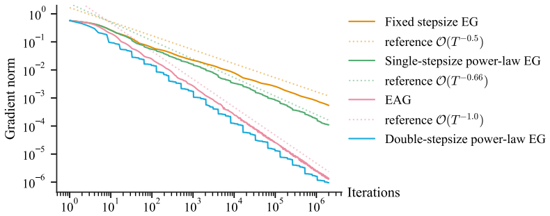
For unconstrained biaffine min-max optimization, a deterministic dynamic stepsize schedule that follows a discretization of a power-law distribution accelerates the last-iterate convergence of extragradient to O(T^{-2/3+ε}) for any ε > 0 when the same stepsize is used for both extrapolation and update; this rate is tight under that constraint. Allowing distinct stepsizes for the two steps further improves the guarantee to the near-optimal O(T^{-1+ε}). The same construction and analysis apply to the optimistic gradient method.
What carries the argument
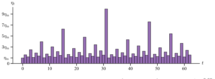
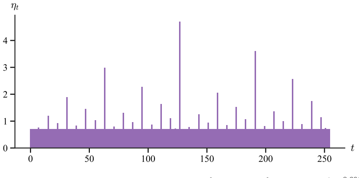
The power-law stepsize schedule obtained by reducing stepsize selection to an auxiliary optimization problem and taking a discretization of its solution.
If this is right
- Extragradient achieves O(T^{-2/3+ε}) last-iterate convergence using only dynamic stepsizes.
- The O(T^{-2/3+ε}) rate is tight when extrapolation and update must share the same stepsize.
- Separate stepsizes for extrapolation and update raise the rate to O(T^{-1+ε}).
- The construction and analysis carry over directly to the optimistic gradient method.
Where Pith is reading between the lines
- The reduction of stepsize choice to an auxiliary optimization problem may be reusable for other first-order methods.
- The same family of schedules could be tested on stochastic or constrained min-max problems to check robustness.
- Practical implementations in game-solving or adversarial training could adopt the schedule for faster last-iterate behavior.
Load-bearing premise
The min-max problem is unconstrained and biaffine, with payoff linear in each player's variables when the other is fixed, and the stepsize schedule must be chosen deterministically in advance using only the iteration horizon.
What would settle it
Running extragradient with the proposed power-law schedule on a concrete biaffine game and checking whether the last-iterate distance to equilibrium decays at a rate slower than T to the power of minus two-thirds.
Figures
read the original abstract
We revisit the convergence guarantees of the Extragradient (EG) method for unconstrained biaffine min-max optimization. It is known that EG with a fixed stepsize achieves a $\Theta(T^{-1/2})$ last-iterate convergence rate, which is slower than the optimal $\mathcal{O}(T^{-1})$ rate attainable by incorporating additional mechanisms such as anchoring. Motivated by recent advances showing that dynamic stepsizes alone can significantly accelerate gradient descent, we ask whether dynamic stepsizes can similarly accelerate the last-iterate convergence of EG. We present the first positive result in this direction. Specifically, we provide a deterministic dynamic stepsize schedule that accelerates the convergence rate of EG to $\mathcal{O}(T^{-2/3+\varepsilon})$ for any $\varepsilon > 0$. We also show that this rate is tight when the extrapolation and update steps of EG use the same stepsize. We then show that allowing different stepsizes for the extrapolation and update steps further improves the convergence rate to the near-optimal $\mathcal{O}(T^{-1+\varepsilon})$. Our analysis reduces stepsize scheduling to an optimization problem, whose solution leads to a stepsize schedule that follows (a discretization of) a power-law distribution. Our proposed stepsize schedules and analysis extend to other methods, such as Optimistic Gradient (OG), and suggest broader applicability to general min-max optimization problems.
Editorial analysis
A structured set of objections, weighed in public.
Referee Report
Summary. The paper claims that for unconstrained biaffine min-max optimization, a deterministic dynamic stepsize schedule derived from an auxiliary optimization problem and taking the form of a power-law discretization accelerates the last-iterate convergence of Extragradient (EG) from the standard Θ(T^{-1/2}) to O(T^{-2/3+ε}) for any ε>0 when the same stepsize is used for extrapolation and update steps; this rate is shown to be tight. Allowing distinct stepsizes for the two steps further improves the rate to the near-optimal O(T^{-1+ε}). The same approach extends to Optimistic Gradient (OG). The schedules depend only on the horizon T and ε, with no other instance-specific knowledge required.
Significance. If the central claims hold after clarification, the work would be significant for showing that dynamic stepsizes alone (without anchoring or other mechanisms) can accelerate last-iterate convergence in min-max settings, via a novel reduction of scheduling to an auxiliary scalar optimization problem whose solution yields a power-law form. The tightness result for the equal-stepsize case and the extension to OG are additional strengths. The approach suggests broader applicability to general min-max problems.
major comments (3)
- [Abstract and stepsize definition (§3–4)] Abstract and the stepsize definition (likely §3–4): The manuscript asserts a deterministic schedule depending only on T and ε that works uniformly for every unconstrained biaffine instance. Standard EG analysis, however, requires each extrapolation and update stepsize η_t to satisfy η_t ≲ 1/L where L is the Lipschitz constant of the monotone operator. Because L is instance-specific and unknown in advance, a single power-law schedule fixed without reference to L cannot simultaneously satisfy stability on large-L instances and achieve the claimed exponent on small-L instances. This is load-bearing for the central claim of instance-independent acceleration.
- [Auxiliary optimization problem (§4)] The auxiliary optimization problem whose solution yields the power-law schedule (likely §4): The reduction is presented as producing a schedule that delivers the stated rates, yet the formulation of this auxiliary problem is not shown to enforce the EG stability bound uniformly across L. If the problem is solved after implicitly setting L=1 or absorbing L into constants that must later be tuned per instance, the claimed O(T^{-2/3+ε}) guarantee does not follow for arbitrary problems from the given deterministic schedule.
- [Main convergence theorem] Theorem establishing the O(T^{-2/3+ε}) rate (likely the main convergence theorem): The proof must explicitly track how the power-law exponents and leading coefficients interact with the biaffine operator norm; without this, it is impossible to verify that the last-iterate error bound holds independently of L rather than under a hidden normalization.
minor comments (2)
- [Introduction] The precise statement of the biaffine payoff and the unconstrained setting could be given an explicit equation early in the introduction for clarity.
- [Notation and improved-rate section] Notation for the two distinct stepsizes (when they differ) should be introduced consistently before the improved-rate theorem.
Simulated Author's Rebuttal
We thank the referee for their careful and constructive review of our manuscript. The comments highlight an important point regarding the Lipschitz constant that requires clarification in the presentation. We provide point-by-point responses below and will make the suggested revisions to improve the manuscript.
read point-by-point responses
-
Referee: [Abstract and stepsize definition (§3–4)] The manuscript asserts a deterministic schedule depending only on T and ε that works uniformly for every unconstrained biaffine instance. Standard EG analysis, however, requires each extrapolation and update stepsize η_t to satisfy η_t ≲ 1/L where L is the Lipschitz constant of the monotone operator. Because L is instance-specific and unknown in advance, a single power-law schedule fixed without reference to L cannot simultaneously satisfy stability on large-L instances and achieve the claimed exponent on small-L instances. This is load-bearing for the central claim of instance-independent acceleration.
Authors: We agree that the stability condition involving the Lipschitz constant L must be carefully addressed. Our results are derived under the normalization L = 1, which is a standard assumption in convergence analyses of first-order methods to focus on the rate in terms of T. The deterministic power-law schedule is obtained for this normalized setting and therefore depends solely on T and ε. We will revise the abstract and sections 3–4 to explicitly state the normalization assumption L=1 and clarify that the instance-independence holds for normalized biaffine operators. For unnormalized instances, scaling the stepsizes by 1/L would be needed if L were known, but the exponent of the rate remains unchanged. This revision will make the scope of the claims precise. revision: yes
-
Referee: [Auxiliary optimization problem (§4)] The auxiliary optimization problem whose solution yields the power-law schedule (likely §4): The reduction is presented as producing a schedule that delivers the stated rates, yet the formulation of this auxiliary problem is not shown to enforce the EG stability bound uniformly across L. If the problem is solved after implicitly setting L=1 or absorbing L into constants that must later be tuned per instance, the claimed O(T^{-2/3+ε}) guarantee does not follow for arbitrary problems from the given deterministic schedule.
Authors: The auxiliary optimization problem is set up under the normalization L=1, with the stability constraint η_t < 1 incorporated into the formulation. The power-law solution is chosen to satisfy this bound while optimizing the convergence exponent. We will update section 4 to include a clear statement of the normalization and demonstrate that the resulting schedule respects the stability condition for L=1. This ensures the claimed rates apply to the normalized problems as stated. revision: yes
-
Referee: [Main convergence theorem] Theorem establishing the O(T^{-2/3+ε}) rate (likely the main convergence theorem): The proof must explicitly track how the power-law exponents and leading coefficients interact with the biaffine operator norm; without this, it is impossible to verify that the last-iterate error bound holds independently of L rather than under a hidden normalization.
Authors: The proof of the main theorem assumes the biaffine operator has unit norm (L=1) and derives the last-iterate bound accordingly, with the power-law parameters chosen to optimize under the stability constraint. The leading coefficients are selected to ensure the bound holds independently of other instance parameters under this normalization. We will revise the theorem and its proof to explicitly reference the normalization and detail the interaction with the operator norm, making the analysis fully transparent. revision: yes
Circularity Check
No circularity; derivation reduces scheduling to auxiliary optimization without self-reference or fitted inputs
full rationale
The paper states that its analysis reduces stepsize scheduling to an auxiliary optimization problem whose solution is a power-law discretization; this is a direct derivation of the schedule from the optimization objective rather than a self-definitional loop, a fitted parameter renamed as prediction, or a load-bearing self-citation. No equations or claims in the provided text equate the claimed O(T^{-2/3+ε}) or O(T^{-1+ε}) rates to the inputs by construction, and the deterministic schedule depending only on T is presented without invoking uniqueness theorems or ansatzes from prior self-work. The central result therefore remains independent of its own outputs.
Axiom & Free-Parameter Ledger
free parameters (1)
- ε > 0
axioms (2)
- domain assumption The payoff function is biaffine (linear in each block when the other is fixed).
- domain assumption Stepsize schedule can be chosen deterministically from the horizon T alone.
Reference graph
Works this paper leans on
-
[1]
Zihan Zhang, Jason Lee, Simon Du, and Yuxin Chen
ArXiv preprint, 2410.12395. Zihan Zhang, Jason Lee, Simon Du, and Yuxin Chen. Anytime acceleration of gradient descent. InThe Thirty Eighth Annual Conference on Learning Theory, pages 5991–6013. PMLR, 2025. Contents 1 Introduction 1 1.1 Related Works . . . . . . . . . . . . . . . . . . . . . . . . . . . . . . . . . . . . . 5 2 Preliminary 6 3 Main results...
-
[2]
Also, when ρ= 3− √ 7 2 , direct calculation shows z1 = 1
Indeed, the function ρ7→z 1 = 1 2 2−ρ− p 4ρ−ρ 2 is monotonically decreasing on(0, 3− √ 7 2 ), because bothρ7→ρ and ρ7→4ρ−ρ 2 are monotonically increasing. Also, when ρ= 3− √ 7 2 , direct calculation shows z1 = 1
-
[3]
Lemma A.5.The Riemann zeta function ζ(z) = ∞X n=1 1 nz = 1 1z + 1 2z + 1 3z +· · · is monotonically decreasing on(1,∞)and satisfiesζ(z)<1 + 1 z−1
The claim is thus proved. Lemma A.5.The Riemann zeta function ζ(z) = ∞X n=1 1 nz = 1 1z + 1 2z + 1 3z +· · · is monotonically decreasing on(1,∞)and satisfiesζ(z)<1 + 1 z−1 . Proof. Monotonicity comes from the monotonicity of each term in the summation. The upper bound is proved with an integral, ζ(z) = 1 + ∞X n=2 1 nz <1 + ∞X n=2 Z n n−1 1 xz dx = 1 + Z ∞...
-
[4]
, r} , {z(i) t }t∈N is a trajectory generated by EG with the same stepsize sequence on the instance(X i,Y i, ℓi)
for each i∈ {1, . . . , r} , {z(i) t }t∈N is a trajectory generated by EG with the same stepsize sequence on the instance(X i,Y i, ℓi). Proof. As ℓ is bilinear, we define A to be its matrix, i.e., ℓ(x, y) =x TAy. Let r= rank(A) and A= Pr i=1 σiuivT i be the singular value decomposition (SVD) ofA, and {u1, . . . , un},{v 1, . . . , vm} be two sets of ortho...
-
[5]
For all values ofβstrictly larger than 3 2, we have Iβ(s) =I β(0)− Z s 0 ln(1−t+t 2)t−β/2−1dt ≤I β(0) + Z s 0 t·t −β/2−1dt(−ln(1−t+t 2)≤twhenevert≥0) =I β(0) + Z s 0 t−β/2dt=I β(0) + s1−β/2 1−β/2 .(23) 26 Therefore, for any β > 3 2, we have Iβ(0)<0 , and it is possible to choose a sufficiently small ηm such that Iβ((ηma/L)2)<0 for all a∈[0, L] . We are no...
-
[6]
Because η2 mb2 ∈[0, 1 2], we have p· β 2−β (ηmb)2 + (1−p) ln 1−η 2 mb2 +η 4 mb4 ≤ p· β 2−β −(1−p)· 1 2 (ηmb)2, and this value is nonpositive whenp≤ 2−β 2+β
If we substitute b= a L and apply (23), we have Eη∼E ln(1−η 2a2 +η 4a4) =p· β 2 (ηmb)βIβ((ηmb)2) + (1−p) ln 1−η 2 mb2 +η 4 mb4 ≤p· β 2 (ηmb)β Iβ(0) + (ηmb)2−β 1−β/2 + (1−p) ln 1−η 2 mb2 +η 4 mb4 ≤ pβ·I β(0) 2 (ηmb)β +p· β 2−β (ηmb)2 + (1−p) ln 1−η 2 mb2 +η 4 mb4 .(26) The function ln(1−z+z 2) is convex on [0, 1 2], has a value of 0 when z= 0 , and has a v...
-
[7]
Define a∗ =T −1/β
Letβ= ( 2 3 +ε) −1 ∈( 4 3 , 3 2). Define a∗ =T −1/β. Consider a Pareto distribution A with shape β truncated on [a∗,1] . Specifically, we have forx∈[a ∗,1], dA(x) = 1 V x−β−1dx, whereVis the normalizing constantV= R 1 a∗ a−β−1da= (a −β ⋆ −1)/β= (T−1)/β. In the next steps, we will prove that Ea∼A h lna+ T 2 Eη∼E ln(1−a 2η2 +a 4η4) i ≥lnC− 2 3 +ε lnT. We fi...
-
[8]
We finally can substitute it back into (29), T 2 Ea∈A[ln(1−a 2η2 +a 4η4)] = T 4V ·S≥ 2T Cβ 2 ln Iβ(0)β2 8 = 2T β(T−1) ln Iβ(0)β2 8
Therefore, S≥min n −1, 8 β2 ln Iβ(0)β2 8 o = 8 β2 ln Iβ(0)β2 8 . We finally can substitute it back into (29), T 2 Ea∈A[ln(1−a 2η2 +a 4η4)] = T 4V ·S≥ 2T Cβ 2 ln Iβ(0)β2 8 = 2T β(T−1) ln Iβ(0)β2 8 . Therefore, Ea∼A lna+ T 2 Eη∼E[ln(1−a 2η2 +a 4η4)] =E a∼A[lna] + T 2 Eη∼E,a∼A ln(1−a 2η2 +a 4η4) ≥ 1 β − T β(T−1) lnT+ 2T β(T−1) ln Iβ(0)β2 8 =− 1 β lnT+ 1 β h ...
-
[9]
=−2 ln 2, so 2 ln(1−t)>−4 ln 2·t . Therefore, fors∈(0, 1 2], Iρ,β(s) =I ρ,β(0)− Z s 0 ln(1 + (ρ−2)t+t 2)t−β/2−1dt ≤I ρ,β(0) + Z s 0 (4 ln 2·t)t −β/2−1dt =I ρ,β(0) + 4 ln 2 Z s 0 t−β/2dt=I ρ,β(0) + 4 ln 2 1−β/2 s1−β/2.(35) Let λm = min n (1− β 2 ) −Iρ,β(0) 8 ln 2 1/(2−β) , 1√ 2 o >0 ; the value satisfies λ2 m ≤ 1 2 and the following equality: 4 ln 2 1−β/2 ...
-
[10]
and (35). Then, we plug this into (34) and obtain Eλ∼E ln(1 + (ρ−2)λ 2a2 +λ 4a4) = β 2 λma L βZ ∞ (λma/L)2 ln(1 + (ρ−2)t+t 2)t−β/2−1dt = β 2 λma L β Iρ,β (λma/L)2 ≤ β 2 λma L β Iρ,β(0) 2 , 33 which can be combined with (33) to get lnR ρ,T (E, a)≤lnL+ ln a L + T 2 β 2 λma L β Iρ,β(0) 2 = lnL+ lnb+ T 2 β 2 (λmb)β Iρ,β(0) 2 (substituteb= a L) ≤lnL− 1 β lnT− ...
-
[11]
Substituting b= a L and applying (35), we have Eλ∼E ln(1−(ρ−2)λ 2a2 +λ 4a4) =p· β 2 (λmb)βIρ,β((λmb)2) + (1−p) ln 1 + (ρ−2)λ 2 mb2 +λ 4 mb4 ≤p· β 2 (λmb)β Iρ,β(0) + 4 ln 2 1−β/2 (λmb)2−β + (1−p) ln 1 + (ρ−2)λ 2 mb2 +λ 4 mb4 ≤ pβ·I ρ,β(0) 2 (λmb)β +p· 4 ln 2·β 2−β (λmb)2 + (1−p) ln 1 + (ρ−2)λ 2 mb2 +λ 4 mb4 .(36) Assuming ρ≤ 1 6 < 3− √ 7 2 ; Lemma A.4 guar...
-
[12]
In the last step, we used the fact that if x∈R, y∈[0,1) , then |⌈x−y⌉ −x| ≤1 (Lemma A.2)
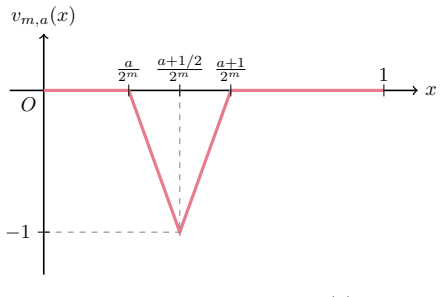
Therefore, |En(vm,a)|= 1 n n−1X i=0 vm,a(φi)− Z 1 0 vm,a(x)dx = 1 n S n 2m −Φ 2(a) −(−2 −m−1) = 1 n S n 2m −Φ 2(a) + 1 2 · n 2m = 1 n S n 2m −Φ 2(a) + 1 2 n 2m −Φ 2(a) + 1 n 1 2 n 2m −Φ 2(a) − 1 2 · n 2m ≤ 1 2n + 1 2n n 2m −Φ 2(a) − n 2m ≤ 1 n . In the last step, we used the fact that if x∈R, y∈[0,1) , then |⌈x−y⌉ −x| ≤1 (Lemma A.2). D.3 Bibliographic not...
1935
-
[13]
It is the integral of the Haar wavelets [Haar, 1910]
and Schauder [1927]. It is the integral of the Haar wavelets [Haar, 1910]. Along with linear functions, it forms a countable basis of C[0,1] . The exact form of this decomposition lemma appears in Ul’yanov [1972]. The system is useful in decomposing a function into local, simpler parts, akin to Fourier and wavelet transforms. We refer the readers to Kashi...
1927
-
[14]
If|f(x)| ≤Mon[x, x+ 2δ], then ∆2 δf(x) ≤4M
-
[15]
If f is M-Lipschitz continuous on [x, x+ 2δ] , then ∆2 δf(x) ≤2M δ ; as a consequence, if f is continuous on [x, x+ 2δ] and |f ′(x)| ≤M on (x, x+ 2δ) , then the same bound holds
-
[16]
Proof.The zeroth-order statement can be proved with the triangle inequality ∆2 δf(x) ≤ |f(x)|+ 2|f(x+δ)|+|f(x+ 2δ)| ≤M+ 2M+M= 4M
If f ′ is continuous on [x, x+ 2δ] and |f ′′(x)| ≤M on (x, x+ 2δ) , then ∆2 δf(x) ≤M δ 2. Proof.The zeroth-order statement can be proved with the triangle inequality ∆2 δf(x) ≤ |f(x)|+ 2|f(x+δ)|+|f(x+ 2δ)| ≤M+ 2M+M= 4M. The first-order statement can be proved with the triangle inequality ∆2 δf(x) =|(f(x+ 2δ)−f(x+δ))−(f(x+δ)−f(x))| ≤ |f(x+ 2δ)−f(x+δ)|+|f(x...
-
[17]
Forz >0, ℓψ(z) = 2 lnz+ℓ ψ(1/z).(41)
-
[18]
Forz∈[0,1], −2 ln(sinψ) −1 ≤ℓ ψ(z)≤0,(42) −4 ln(sinψ) −1 cosψ z≤ℓ ψ(z).(43)
-
[19]
Forz∈(0,1], ℓ′ ψ(z) ≤ 2 sinψ ,(44) ℓ′′ ψ(z) ≤ 2 (sinψ) 2 .(45)
-
[20]
Forz∈(0, 1 2], ℓ′ ψ(z) ≤4,(46) ℓ′′ ψ(z) ≤8,(47)
-
[21]
For (42), observe that fψ is convex and is maximized over [0,1] at an endpoint
The functionℓ ψ has a bounded total variation V 1 0 (ℓψ)≤4 ln(sinψ) −1.(48) Proof.The first statement follows fromf ψ(z) =z 2fψ(1/z). For (42), observe that fψ is convex and is maximized over [0,1] at an endpoint. Since fψ(0) = 1 and fψ(1) = 2−2 cosψ≤1 , we have fψ(z)≤1 for z∈[0,1] ; solving the first-order condition f ′ ψ(z) = 0 yields z∗ = cosψ , so the...
-
[22]
= 5 4 −cosψ≥ 1 4; this proves (46). Similarly, we have ℓ′′ ψ(z) ≤ 1 |z−eiψ|2 + 1 |z−e−iψ|2 = 2 fψ(z) , and (45) and (47) can be proved with again plugging inf ψ(z)≥(sinψ) 2 on[0,1]andf ψ(z)≥ 1 4 on[0, 1 2]respectively. To prove the total variation, we notice that ℓψ is decreasing on the left of z∗ and increasing on the right. Because its range is [−2 ln(s...
-
[23]
+” in the “±
We split all intervals of the form[L a, Ra]fora= 0,1, . . . ,2 m −1into four cases. • Consider all intervals such that {0, σ 2 , σ,2σ} ∩[L a, Ra]̸=∅ . There are at most 7 such intervals; for each such interval, we apply the second condition from Lemma D.11, and using the fact that f is 4 σsinψ -Lipschitz (from (51) and the definition of f), we can bound 1...
-
[24]
and positive on ( 1 4 ,+∞) . Similar to the EG cases, the integral IOG β can be evaluated into a closed form when 1< β <2 ; however, this proof is significantly more complicated and requires special functions; see Lemma A.7, where IOG β (0) is obtained with the substitution s=β/2: IOG β (0) = 2β/2+1π βsin(πβ/4) 4F3 − β 4 , β 12 , β+ 4 12 , β+ 8 12 ; 1, 1 ...
2021
discussion (0)
Sign in with ORCID, Apple, or X to comment. Anyone can read and Pith papers without signing in.