REVIEW 4 major objections 6 minor 1 cited by
Singular Bayesian Neural Networks
T0 review · 4 major / 6 minor · reviewed 2026-08-03 · deepseek-v4-flash
Pith's one-line read This paper argues that Bayesian neural networks can dispense with the O(mn) parameter cost of mean-field posteriors by writing each weight matrix as a product of two small matrices, W = AB^T, which induces a posterior concentrated on the ra
desk verdict Low-rank BNN recipe with solid experiments and a clean convex-hull transfer result, but the covariance-correlation claim is wrong and the main bound's assumptions don't match the implemented method. read the letter →
The pith
A machine-rendered reading of the paper's core claim, the machinery that carries it, and where it could break.
The reading
What carries the argument
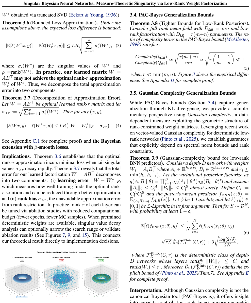
The central object is the induced posterior q_W obtained by pushing a factorized mean-field posterior over factors A and B through the map (A, B) ↦ W = AB^T. Its key property is that the support is exactly the rank-r manifold R_r = {W : rank(W) ≤ r}, which has Lebesgue measure zero in R^{m×n}, making q_W singular with respect to Lebesgue measure. This one construction does three jobs: it reduces variational parameters from 2mn to 2r(m+n) (counting means and variances on both factors), it manufactures off-diagonal covariances among weights that share latent factors, and it makes the posterior's capacity rank-aware. The theoretical results then hang off this construction: PAC-Bayes complexity
What would settle it
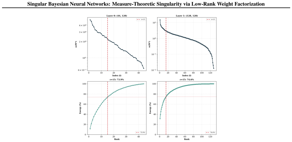
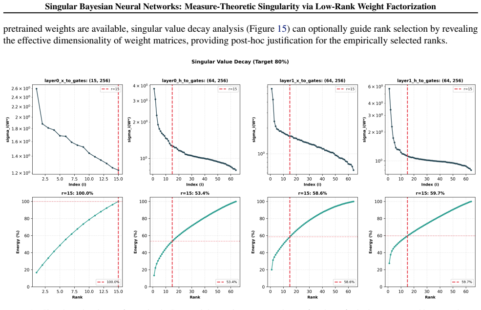
Train the same architecture deterministically, compute the singular values of each weight matrix, and measure the cumulative Frobenius energy retained at the selected rank r. If, for the rank where the low-rank Bayesian model remains competitive, the retained energy falls well below 90%, the rank-bias term in the loss decomposition becomes the dominant error source and the method's theoretical advantage over full-rank baselines would fail to show up as predicted.
Extended reading notes
Core claim
On its own terms, the paper establishes that a variational posterior over low-rank factors A, B — with W = AB^T — induces a distribution over weights that lives entirely on the rank-r manifold, a measure-zero set in R^{m×n}. Because of this geometric restriction, the posterior captures structured correlations between weights (weights sharing latent factors covary), and the complexity term in the PAC-Bayes bound drops from O(mn) to O(r(m+n)). The authors prove that the loss of the low-rank model relative to the full-rank optimum decomposes into an optimization term and a rank-bias term controlled by the tail singular values of the target weight matrix, so fast singular value decay makes the a
Load-bearing premise
The whole scheme leans on the assumption that trained weight matrices have fast singular value decay, so the tail left out by the rank-r factorization is negligible; the paper's own energy-retention plot for a representative LSTM shows rank 15 capturing only about 74% of the total weight energy, so this assumption is doing real work.
Editorial extensions
If this is right
- Low-rank variational BNNs have PAC-Bayes complexity O(sqrt(r(m+n))) rather than O(sqrt(mn)), so in data-limited regimes they generalize better than full-rank mean-field with comparable empirical risk.
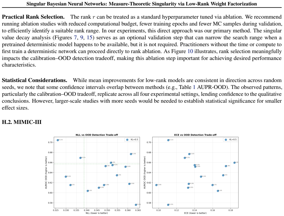
- The loss decomposition gives a concrete rank-selection criterion: inspect the singular value decay of trained weights and choose r where the tail energy is small.
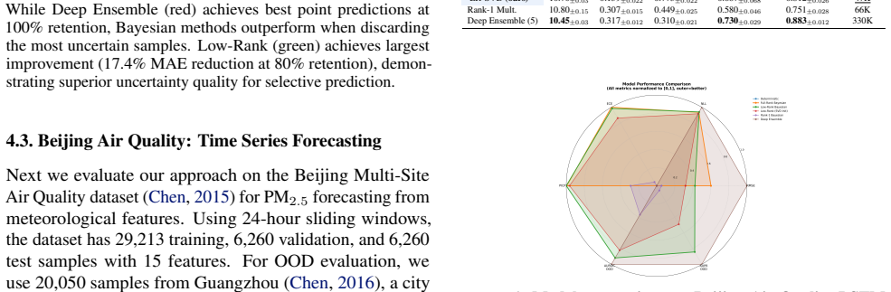
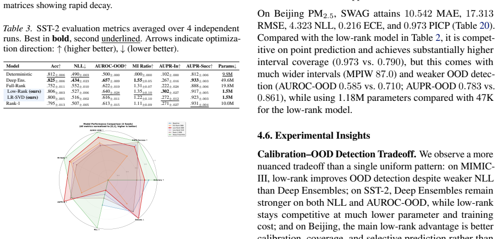
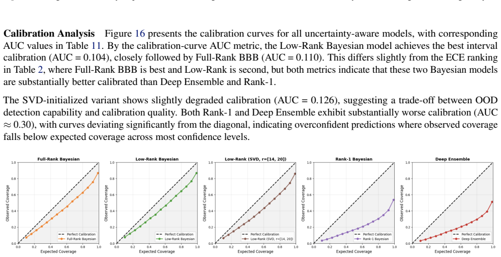
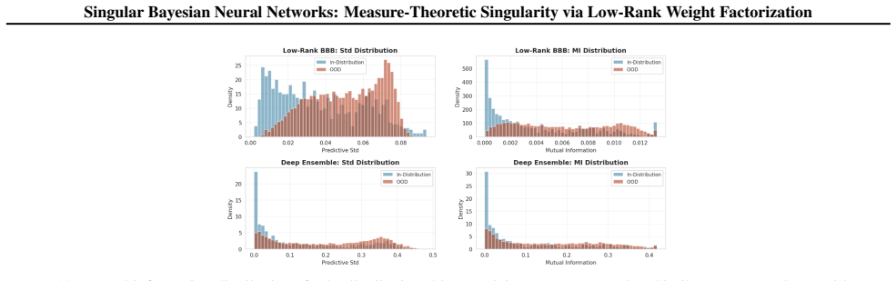
- The induced weight correlations propagate uncertainty coherently across rows and columns, which shows up as improved OOD separation and better selective prediction at 80% retention in the time-series experiments.
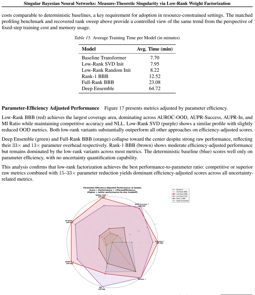
- On the transformer benchmark the method trains in about 8 minutes versus 23 minutes for full-rank BBB and about 65 minutes for a five-member ensemble, making Bayesian inference affordable at scale.
Reading between the lines
- The measure-theoretic singularity suggests a broader recipe: any posterior whose support is a lower-dimensional manifold in weight space buys correlated uncertainty and reduced capacity for free; whether the manifold is the rank-r set or something else (e.g., a subspace or a product manifold) should be a design choice rather than an accident.
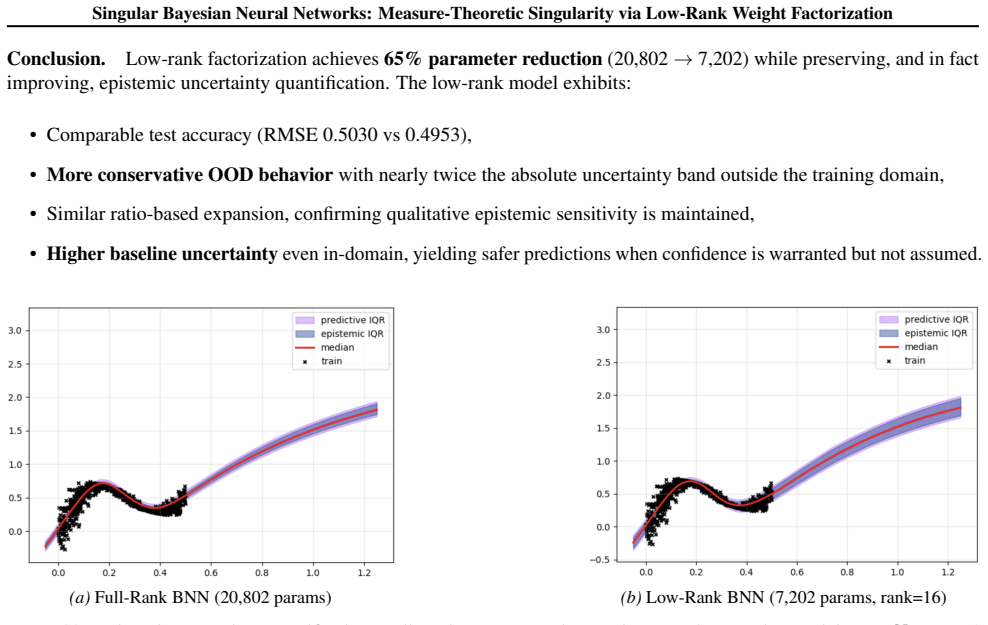
- The convex-hull transfer argument (the posterior-mean predictor's Gaussian complexity is bounded by that of the deterministic low-rank class) implies that ensembling deterministic low-rank networks—or averaging many posterior samples—inherits the same rank-sensitive capacity control, which may explain why the low-rank Bayesian ensemble in the appendix recovers calibration.
- The method becomes testable per layer: if the tail-energy analysis is done adaptively during training, the factorization could choose its own effective rank, making the singular-value-decay assumption self-verifying on each dataset.
- A concrete failure mode to probe is a dataset whose features genuinely live in a high-rank subspace; there the rank-bias term grows and the method should underperform full-rank baselines—an experiment one could run with synthetic data of controlled singular value spectra.
Editorial analysis
A structured set of objections, weighed in public.
Referee Report
Summary. The paper introduces a low-rank variational inference framework for Bayesian neural networks in which each weight matrix is parameterized as W = AB^T with independent mean-field Gaussian posteriors on the factors A and B. The induced posterior on W is singular with respect to Lebesgue measure and supported on the rank-r manifold. The authors derive three theoretical results: a PAC-Bayes bound whose complexity term scales as sqrt(r(m+n)) instead of sqrt(mn), a loss-approximation bound based on the Eckart-Young-Mirsky theorem, and a Gaussian-complexity bound for Bayesian predictive means transferred from deterministic low-rank networks. Empirically, they evaluate the method on MIMIC-III mortality prediction, Beijing PM2.5 forecasting, and SST-2 sentiment classification, reporting competitive predictive performance with substantially fewer parameters than full-rank mean-field VI and deep ensembles, together with improved OOD detection and calibration in several settings.
Significance. If the claims were fully supported, the paper would be a valuable contribution: it offers a parameter-efficient, end-to-end Bayesian treatment of low-rank structure and a useful collection of empirical results across architectures. The empirical core is a real strength: multiple seeds, standard benchmarks, controlled profiling, ablation studies, and honest reporting of overlapping confidence intervals and calibration gaps. The theoretical scaffolding is also potentially useful, but several of its advertised guarantees are currently overclaimed or only conditionally valid. The empirical findings can likely stand independently, but the paper's central narrative that low-rank factorization is 'provably' justified by fast singular value decay needs repair.
major comments (4)
- [Section 3.3 / Figures 7, 9] The paper repeatedly asserts that fast singular value decay 'is verified empirically' (Sections 1, 3.3, Appendix H), but the evidence provided does not support this. Figure 9 shows that for the MIMIC-III MLP layers, rank r=15 captures only 73.9% and 74.6% of Frobenius energy, so the tail quantity sigma_{>r} in Eq. (3) is about 0.51 ||W*||_F. This is not small by any quantitative standard, and the rank-bias term in Eq. (4) can therefore dominate the bound. No threshold is given for what counts as 'fast' decay. The loss-approximation rationale for low-rank substitution is thus not established by the paper's own data. Please either provide a quantitative decay criterion and show it is met, or explicitly state that the loss-bound guarantees are conditional on such decay; the empirical results do not depend on this premise.
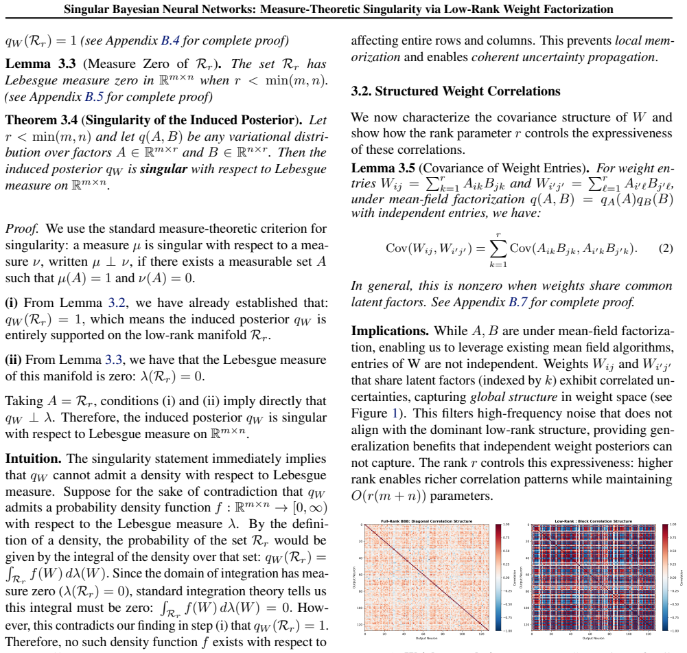
- [Lemma 3.5 / Section 3.2] The covariance interpretation in Lemma 3.5 is too broad and, as stated, misleading. Under q(A,B) = q(A)q(B) with independent entries, the covariance in Eq. (2) is zero for any pair of weights with i != i' AND j != j', because E[A_ik A_i'k] = E[A_ik]E[A_i'k] and E[B_jk B_j'k] = E[B_jk]E[B_j'k]. Nonzero off-diagonal covariance occurs only for pairs sharing the same row index (i = i') or the same column index (j = j'), and even then it is proportional to the mean of the other factor. The statement 'weights sharing latent factors (indexed by k) exhibit correlated uncertainties' overstates the effect: sharing the latent dimension k does not by itself create correlation. The 'global structure' claim in Section 3.2 and the Figure 1 caption should be corrected accordingly.
- [Theorem 3.9 / Assumption E.4] The Gaussian-complexity transfer theorem relies on Assumption E.4: ||A_i||_2 <= C_A^i and ||B_i||_2 <= C_B^i almost surely under the variational posterior. The experiments use ordinary Gaussian variational posteriors with unbounded support and no truncation or spectral projection is reported in the experimental details (Section G). Thus Theorem 3.9 as stated does not apply to the actual predictor implemented in the paper. Appendix E.10 provides a high-probability relaxation, but it requires an additional convexity assumption and is not presented in the main text. Please either enforce the bounded-support assumption (e.g., by truncation or spectral normalization) and document it, or reposition Theorem 3.9 as a conditional theoretical contribution that is distinct from the experimental protocol.
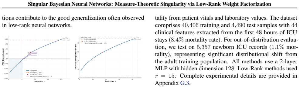
- [Theorem 3.8 / Eq. (5)] The claim of 'provably tighter generalization bounds' is based only on the ratio of the KL complexity terms. A PAC-Bayes bound is the sum of an empirical-risk term and a complexity term; a smaller complexity coefficient does not by itself guarantee a numerically tighter bound unless the empirical risks are comparable. Figure 3 already shows that the PAC-Bayes bound becomes vacuous above a critical rank, so the 'provably tighter' language should be qualified. This is not a blocking issue, but the abstract and Section 3.4 should avoid implying that the parameter-count reduction immediately yields a uniformly tighter generalization certificate.
minor comments (6)
- [Section 3.4, Eq. (5)] The notation 'simeq' in Eq. (5) is imprecise. For equal per-parameter KL constants C_max, the ratio is exactly sqrt(r(1/din + 1/dout)); please state the equality conditions.
- [Section 3.3] The paper calls W* the 'optimal full-rank weight matrix (learned via back-propagation)' in a Bayesian setting; clarify that this is the deterministic empirical-risk minimizer, not a Bayesian posterior quantity.
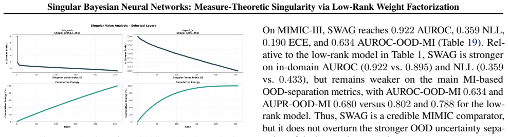
- [Figure 7 caption] The caption says 'rapid decay', but no quantitative notion of 'rapid' is provided. Suggest replacing with a numerical description of the decay (e.g., energy retention at selected ranks).
- [Section 4.5 / Appendix H.6] The SWAG comparisons are useful, but the main-text summary would benefit from a clearer statement that these runs use different numbers of seeds and slightly different evaluation protocols than the main tables; the appendix already does this well.
- [General / formatting] There is a missing comma in the author line (Toure1 David A. Stephens 1) and the PMLR line appears as 'PMLR 306, 2026' with inconsistent spacing; minor typographical cleanup is needed.
- [Appendix H.4.1 / Table 4] Table 4 is based on a single profiling run per method. This is fine as a controlled benchmark, but adding a sentence in the main text that these are single-run measurements would prevent overinterpretation.
Circularity Check
No significant circularity; the paper's theoretical results follow from standard external theorems, definitional counting, and explicit inclusion arguments rather than from fitted inputs or self-citations.
full rationale
The main claimed derivations are self-contained in the relevant sense. Theorem 3.4's singularity result is a direct measure-theoretic consequence of the parameterization W=AB^T: the pushforward posterior satisfies q_W(R_r)=1 because rank(AB^T)<=r by construction, and R_r has Lebesgue measure zero by a standard polynomial-zero-set argument. This is immediate from the definitions, but it is not circular reasoning: the proof establishes the claimed support property rather than assuming it. The loss approximation theorems (Theorems 3.6 and 3.7) rely on the L-Lipschitz/bounded-input assumptions and the external Eckart-Young-Mirsky theorem; the rank-bias term sigma_{>r} is defined from W* and is not fitted from the data used to evaluate the bound. The PAC-Bayes result (Theorem 3.8) reduces to counting D_full=mn versus D_LR=r(m+n) parameters and applying standard KL factorization; the reported sqrt(r(1/m+1/n)) ratio is algebraic. The Gaussian complexity transfer (Theorem 3.9) uses an external bound from Pinto et al. (2025) and a genuine inclusion argument: the posterior-mean predictor lies in the closed convex hull of the support class, and Gaussian complexity is invariant under convex hull and closure. No load-bearing self-citations were identified; citations to Blundell, Fortunato, Dusenberry, and Pinto are external prior work, not self-referential uniqueness claims. The empirical claim of 'fast singular value decay' is arguably weakly supported by the paper's own Figure 9 (about 74% energy at r=15), but that is a correctness/evidence concern about an empirical premise, not a reduction of a predicted quantity to a fitted input. Likewise, the acknowledged limitations (calibration gap, overlapping confidence intervals, single-run ensembling study) are empirical caveats, not circular steps. The score is therefore 0.
Assumptions & free parameters
free parameters (3)
- rank r per layer =
r=15 (MIMIC), r=[14,20] (Beijing), r=16 (SST-2)
- KL scale beta =
0.5/N_batches (MIMIC), 0.09/N_train (Beijing), 0.001/N_batches (SST-2)
- Spectral norm bounds C_A, C_B =
Not specified
assumptions (6)
- standard math Eckart-Young-Mirsky theorem
- standard math McAllester PAC-Bayes inequality
- domain assumption Pinto et al. (2025) Gaussian complexity bounds for low-rank deterministic networks
- domain assumption Loss is L-Lipschitz and inputs are bounded by R
- domain assumption Fast singular value decay of weight matrices
- ad hoc to paper Assumption E.4: variational posterior support bounded in spectral norm almost surely
Cite this review
Pith. "Pith review of Singular Bayesian Neural Networks." pith.science (2026). https://pith.science/paper/ZNNHJ52F
@misc{pith2026260200387,
  author       = {Pith},
  title        = {Pith review of: Singular Bayesian Neural Networks},
  year         = {2026},
  howpublished = {\url{https://pith.science/paper/ZNNHJ52F}},
  note         = {Machine review of arXiv:2602.00387}
}
abstract
Bayesian neural networks promise calibrated uncertainty but require $O(mn)$ parameters for standard mean-field Gaussian posteriors. We argue this cost is often unnecessary, particularly when weight matrices exhibit fast singular value decay. By parameterizing weights as $W = AB^{\top}$ with $A \in \mathbb{R}^{m \times r}$, $B \in \mathbb{R}^{n \times r}$, we induce a posterior that is \emph{singular} with respect to the Lebesgue measure, concentrating on the rank-$r$ manifold. This singularity captures structured weight correlations through shared latent factors, geometrically distinct from mean-field's independence assumption. We derive PAC-Bayes generalization bounds whose complexity term scales as $\sqrt{r(m+n)}$ instead of $\sqrt{m n}$, and prove loss bounds that decompose the error into optimization and rank-induced bias using the Eckart-Young-Mirsky theorem. We further adapt recent Gaussian complexity bounds for low-rank deterministic networks to Bayesian predictive means. Empirically, across MLPs, LSTMs, and Transformers on standard benchmarks, our method achieves competitive predictive performance while using up to $33\times$ fewer parameters than 5-member Deep Ensembles. It substantially improves OOD detection and often improves calibration relative to mean-field and perturbation baselines, while Deep Ensembles can still be stronger on in-distribution likelihood-based metrics.
Figures
Figures from the paper (17 more)




Forward citations
Cited by 1 Pith paper
-
Not Just How Much, But Where: Decomposing Epistemic Uncertainty into Per-Class Contributions
Per-class epistemic uncertainty decomposes mutual information as C_k = Var[p_k]/(2 μ_k), enabling class-specific deferral and shift detection.
Reference graph
Works this paper leans on
-
[1]
This depends on optimization quality and can be reduced with better training procedures
Learning error: ∥W−W ∗ r ∥F measures how far the learned W=AB ⊤ is from the optimal rank-r approximation. This depends on optimization quality and can be reduced with better training procedures
-
[2]
ln QD i=1 qi(θi) QD i=1 pi(θi) # =E θ∼Q
Rank bias (approximation error): qPρ i=r+1 σ2 i (W ∗) is the unavoidable error from restricting to rank r. If W ∗ has rapidly decaying singular values, this term is small. C.4. Extension to Stochastic Weights (Bayesian Setting) Lemma C.7(Variance and Loss, Lemma 1.2.3 in (Nesterov, 2018)).Assume ℓ(·, y)is differentiable and β-smooth in its first argument....
2018
-
[3]
No degradation occurs in the complexity bound from the deterministic to the Bayesian setting. E.7. Generalization from Vector-Valued Gaussian Complexity We now state the generalization theorem from Pinto et al. (2025) for vector-valued Gaussian complexity and Lipschitz losses, which we will apply to our BNN predictor. Theorem E.15(Generalization via vecto...
2025
-
[4]
original class)
The BNN predictor class has the same Gaussian complexity as the support class, despite being a much larger set (closed convex hull vs. original class)
-
[5]
The complexity is bounded by that of Pinto’s deterministic class, allowing us to invoke existing deterministic bounds
-
[7]
A contraction inequality showing that Lipschitz losses contract the vector-valued Gaussian complexity by at most√ πL
-
[8]
We cite it in this combined form to avoid re-deriving technical constants
A concentration inequality relating the empirical Gaussian complexity to generalization. We cite it in this combined form to avoid re-deriving technical constants. Our contribution is the class inclusion argument (Proposition E.13) that enables applying this theorem tof BNN. E.7.1. EXPLICITCOMPLEXITYBOUND FORPINTO’SCLASS We now recall the explicit upper b...
2025
-
[9]
3.Depth dependence: The product QD i=j+1 C0Ci shows how spectral norms accumulate through the network depth
Data dependence: The bound explicitly depends on ∥X∥ F , the norm of the training inputs, unlike PAC-Bayes bounds which depend on the posterior-prior KL divergence. 3.Depth dependence: The product QD i=j+1 C0Ci shows how spectral norms accumulate through the network depth
Show all 28 references
-
[10]
This is an artifact of the layer-peeling proof technique (specifically, how the chaining argument handles the input layer), not a reflection of a missing rank constraint
First layer: The term B1 √h1 for the first layer differs in form from the p rjhj terms for deeper layers. This is an artifact of the layer-peeling proof technique (specifically, how the chaining argument handles the input layer), not a reflection of a missing rank constraint. ...
2025
-
[11]
In the extreme case of a near-deterministic posterior, the PAC-Bayes gap approaches zero while the Gaussian complexity bound remains fixed by the class geometry
Posterior concentration:When the posterior is highly concentrated around a good solution, Cmax can be very small, making the KL term tight. In the extreme case of a near-deterministic posterior, the PAC-Bayes gap approaches zero while the Gaussian complexity bound remains fixe...
-
[12]
The Gaussian complexity bound’s leading term grows linearly in∥X∥ F
Large input norms:PAC-Bayes bounds do not depend on ∥X∥ F , which is advantageous when inputs have very large norm or heavy tails. The Gaussian complexity bound’s leading term grows linearly in∥X∥ F
-
[13]
When din ≫d out and C 2 0 C 4 1 R2 is large, PAC-Bayes can still be favorable despite thedin term, because it avoids the spectral norm constants entirely
High-dimensional inputs with moderate rank:Looking at the full expressions, PAC-Bayes scales with r(din +d out) while Gaussian complexity (with bounded inputs) scales with C 2 0 C 4 1 R2 ·r dout. When din ≫d out and C 2 0 C 4 1 R2 is large, PAC-Bayes can still be favorable des...
-
[14]
Diffuse posteriors with bounded spectral norms:When Cmax is large (the posterior has not concentrated tightly), the PAC-Bayes KL term can be vacuous. The Gaussian complexity bound depends on the spectral norm constraints C1, not on posterior concentration, and can remain infor...
-
[15]
This is the regime where the Gaussian complexity bound is numerically tighter
Normalized inputs with small spectral norm constants:When ∥xj∥2 ≤R with R moderate and spectral norms are well-controlled (C1 not too large), the Gaussian complexity bound’s leading constant √ πLC 0C 2 1 R can be smaller than p Cmax/2. This is the regime where the Gaussian com...
-
[16]
This makes them valuable as aprior-free sanity check
No prior specification required:Unlike PAC-Bayes, which requires choosing a prior P and where the bound quality depends sensitively on this choice, Gaussian complexity bounds depend only on the realized network architecture and data. This makes them valuable as aprior-free san...
-
[17]
good event
Architectural transparency:The bound explicitly shows how rank, spectral norms, and layer dimensions interact through the network depth, providing guidance for architectural design that is not available from the PAC-Bayes bound’s KL-divergence summary. RemarkE.25 (Rank depende...
2017
-
[18]
In reparameterized variational inference, the same clipping can be applied to sampled factors
Projection / spectral normalization.After each parameter update during optimization, rescale factors to enforce spectral norm constraints: Ai ←min 1, C A i ∥Ai∥2 Ai, B i ←min 1, C B i ∥Bi∥2 Bi. In reparameterized variational inference, the same clipping can be applied to sampl...
-
[19]
For example, a truncated Gaussian with support {A:∥A∥ 2 ≤C A} naturally satisfies the assumption
Compact-support families.Use truncated Gaussians or uniform distributions supported on the spectral norm ball. For example, a truncated Gaussian with support {A:∥A∥ 2 ≤C A} naturally satisfies the assumption. This requires computing the normalization constant, which may be com...
2017
-
[20]
Biases are either stochastic Gaussians or deterministic (both tested); we report the deterministic-bias variant for parameter efficiency
Full-Rank Gaussian (BBB).Following (Blundell et al., 2015), we place an independent diagonal Gaussian variational posterior on each weight and bias: q(Wij |µ ij, σ2 ij) =N(µ ij, σ2 ij), reparameterized as W=µ+σ⊙ϵ with ϵ∼ N(0, I). Biases are either stochastic Gaussians or deter...
2015
-
[21]
Each entry of A and B has a diagonal Gaussian posterior: q(Aik) =N(µ A ik,(σ A ik)2) and similarly for B
Low-Rank Gaussian Factorization.We impose a rank- r factorization W≈AB ⊤ where A∈R n×r and B∈R m×r with r≪min(n, m) . Each entry of A and B has a diagonal Gaussian posterior: q(Aik) =N(µ A ik,(σ A ik)2) and similarly for B. The bias remains deterministic. We sweep ranks r∈ {10...
-
[22]
Rank-1 Multiplicative (Dusenberry et al., 2020).Following Dusenberry et al. (Dusenberry et al., 2020a), we fix a deterministic base weight matrix Wand apply a rank-1 stochastic multiplicative perturbation: W ′ = W⊙(s⊗r), where s∈R n and r∈R m are stochastic vectors with diagon...
2020
-
[23]
This prior encourages sparsity by placing probability mass on both a standard Gaussian and a narrow Gaussian; it is identical across all four models to ensure fair comparison
+ (1−π)N(0, σ 2 2), with fixed hyperparameters π= 0.5 , σ1 = 1.0, and σ2 = exp(−6)≈0.00248 . This prior encourages sparsity by placing probability mass on both a standard Gaussian and a narrow Gaussian; it is identical across all four models to ensure fair comparison. Training...
2017
-
[24]
Prior: mixturep(w) = 0.5N(0,2.0 2) + 0.5N(0, e−6)
Full-Rank BNN (Bayes by Backprop):All weights have diagonal Gaussian posteriors q(w) =N(µ w, σ2 w). Prior: mixturep(w) = 0.5N(0,2.0 2) + 0.5N(0, e−6). Total trainable parameters:20,802
-
[25]
Input (1→100 ) and output (100→1 ) layers remain full-rank
Low-Rank BNN:Hidden layer ( 100→100 ) uses factorization W≈AB ⊤ with rank r= 16 . Input (1→100 ) and output (100→1 ) layers remain full-rank. Same mixture prior. Total trainable parameters:7,202(65% parameter reduction). Training uses KL annealing (ramped over 760 epochs) andβ...
-
[26]
This is a desirable property for safe prediction
Wider absolute OOD band:Low-rank maintains significantly larger out-of-domain uncertainty ( 0.0940 vs 0.0483), providing more conservative credible intervals where data are absent. This is a desirable property for safe prediction
-
[27]
This shows low-rank preserves the qualitative epistemic sensitivity: uncertainty grows when leaving the training domain
Sharper expansion ratio:Although in-domain uncertainty is higher in low-rank ( 0.0467 vs 0.0254), the OOD/in- domain ratio is nearly identical (2.01× vs 1.90×). This shows low-rank preserves the qualitative epistemic sensitivity: uncertainty grows when leaving the training domain
-
[28]
Rather than under-confident (overfitting) predictions, the low-rank posterior spreads mass more broadly, yielding conservative predictions even in-domain
Stronger in-domain regularization:Low-rank’s higher baseline epistemic IQR ( 0.0467) reflects structured regular- ization from rank constraints. Rather than under-confident (overfitting) predictions, the low-rank posterior spreads mass more broadly, yielding conservative predi...
-
[2015]
DOI: https://doi.org/10.24432/C5JS49. Chen, S. PM2.5 Data of Five Chinese Cities. UCI Machine Learning Repository, 2016. DOI: https://doi.org/10.24432/C52K58. Chen, T., Fox, E., and Guestrin, C. Stochastic gradient Hamiltonian Monte Carlo. InInternational Conference on Machine...
2016 arXiv
Reviewed August 3, 2026 · model on record in the stance chip above.
Discussion (0). Continue with ORCID to comment.