Earth's Infrared Background
Pith reviewed 2026-05-23 01:17 UTC · model grok-4.3
The pith
The Earth's infrared background in OLR is bounded by isotropic fluctuations on scales no larger than 400 km and 2.5 days.
A machine-rendered reading of the paper's core claim, the machinery that carries it, and where it could break.
Core claim
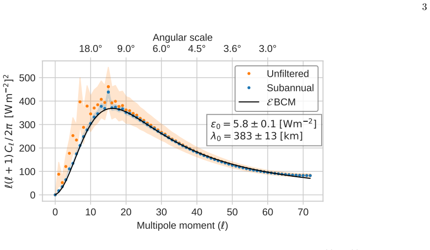
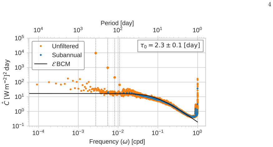
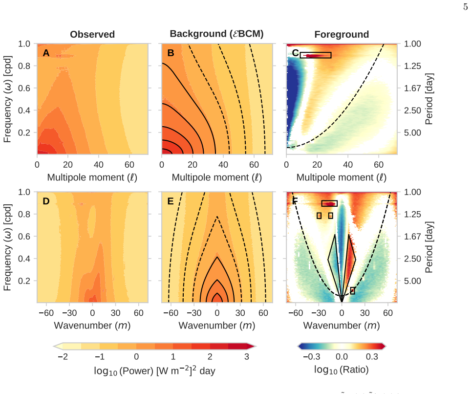
The background is identified as isotropic fluctuations implied by the fluctuation-dissipation theorem in response to internal atmospheric variability on small spatiotemporal scales. A stochastically forced energy balance climate model with a broad-sense red spectrum, first-order in time and second-order in space, is fitted to satellite OLR data, producing an upper bound of about 400 km and 2.5 days on the background fluctuations' spatiotemporal (de)correlations, placing them between meso-scale and synoptic-scale weather.
What carries the argument
A stochastically forced energy balance climate model that is first-order in time and second-order in space, fitted to satellite OLR observations to bound the isotropic background fluctuations.
If this is right
- The fitted model supplies an objective null hypothesis against which waves, storms, and other coherent structures can be isolated in OLR observations.
- Background fluctuations are confined between meso-scale and synoptic-scale weather, so larger-scale features are more likely to be coherent rather than random.
- The model reproduces the observed broad-sense red spectrum of OLR with a simple first-order temporal and second-order spatial process.
- The resulting scale bounds give a concrete reference for what counts as 'background' versus 'signal' in outgoing longwave radiation.
Where Pith is reading between the lines
- The same stochastic-model approach could be applied to other radiation bands or surface variables to test whether similar background scales appear.
- Atmospheric reanalyses or high-resolution simulations could be checked to see whether their small-scale variability matches the reported decorrelation bounds.
- If the bounds hold, operational weather and climate models may need to treat variability below roughly 400 km and 2.5 days as effectively stochastic rather than resolved dynamics.
- The method offers a way to quantify how much of the observed OLR variance must be attributed to internal noise before attributing the rest to external forcing or organized circulation.
Load-bearing premise
The random part of OLR can be fully captured as isotropic fluctuations that follow from the fluctuation-dissipation theorem applied to small-scale internal atmospheric variability.
What would settle it
Satellite OLR records that, after removal of known coherent structures, show statistically significant isotropic correlations persisting well beyond 400 km or 2.5 days while still matching the model's red spectrum would falsify the reported upper bound.
Figures

read the original abstract
Much of the Outgoing Longwave Radiation (OLR) emitted to space is best described as random variability, or the ``Earth's Infrared Background''. A rigorous characterization of this background provides an objective null hypothesis and enables the isolation of atmospheric phenomena -- such as waves, storms, and other coherent structures -- within OLR observations. To this end, we identify the background as isotropic fluctuations implied by the fluctuation-dissipation theorem in response to internal atmospheric variability on small spatiotemporal scales. We use a stochastically forced energy balance climate model, which has a broad sense red spectrum consistent with observations, a first-order process in time, and a second-order process in space. By fitting the model to OLR data from satellite observations, we find that the background fluctuations have an upper bound of about 400~km and 2.5~days on their spatiotemporal (de)correlations, between meso-scale and synoptic-scale weather.
Editorial analysis
A structured set of objections, weighed in public.
Referee Report
Summary. The paper claims that much of the OLR can be described as an 'Earth's Infrared Background' consisting of isotropic fluctuations implied by the fluctuation-dissipation theorem. Using a stochastically forced energy-balance model (first-order in time, second-order in space, red spectrum), the authors fit the model directly to satellite OLR observations and report upper bounds of ~400 km and ~2.5 days on the spatiotemporal decorrelation scales of this background, placing it between meso-scale and synoptic-scale weather. This is positioned as an objective null hypothesis for isolating coherent structures.
Significance. If the central claim holds after addressing the fitting procedure, the result would supply a concrete, observationally calibrated null model for small-scale OLR variability that could aid in the statistical detection of waves, storms, and other organized features. The approach of using a stochastic EBM consistent with red spectra is a standard and defensible choice for this purpose.
major comments (2)
- [Abstract] Abstract: The reported upper bounds (~400 km, ~2.5 days) are obtained by fitting the stochastic EBM parameters directly to the full OLR satellite dataset. The manuscript provides no description of any scale-separation, masking, or filtering step that would isolate the claimed isotropic small-scale background from the longer-correlation coherent structures (waves, storms) also present in the same data. Because the fit necessarily incorporates both components, the resulting scales cannot be guaranteed to bound only the FDT-implied background fluctuations.
- [Abstract] Abstract: No error bars, cross-validation metrics, sensitivity tests to initial conditions or data subsets, or explicit exclusion criteria for the fitted decorrelation scales are supplied. This absence makes it impossible to assess whether the quoted bounds are robust or merely the output of an unconstrained fit to mixed signals.
minor comments (1)
- [Abstract] The abstract states that the model has 'a broad sense red spectrum consistent with observations' but does not cite the specific observational studies or quantify the spectral agreement.
Simulated Author's Rebuttal
We thank the referee for the detailed and constructive report. We address the two major comments point by point below, indicating where revisions will be incorporated.
read point-by-point responses
-
Referee: [Abstract] Abstract: The reported upper bounds (~400 km, ~2.5 days) are obtained by fitting the stochastic EBM parameters directly to the full OLR satellite dataset. The manuscript provides no description of any scale-separation, masking, or filtering step that would isolate the claimed isotropic small-scale background from the longer-correlation coherent structures (waves, storms) also present in the same data. Because the fit necessarily incorporates both components, the resulting scales cannot be guaranteed to bound only the FDT-implied background fluctuations.
Authors: The manuscript fits the stochastic EBM directly to the full OLR dataset without explicit scale separation or masking, as stated in the abstract. We interpret the resulting decorrelation scales as upper bounds on the isotropic background because any contribution from longer-correlated coherent structures would increase the apparent spatiotemporal scales in the fit; the reported values (~400 km, ~2.5 days) are therefore conservative for the FDT-implied background component alone. We will revise the abstract and add a dedicated paragraph in the methods/discussion to explicitly articulate this reasoning and the direction of the bias. revision: partial
-
Referee: [Abstract] Abstract: No error bars, cross-validation metrics, sensitivity tests to initial conditions or data subsets, or explicit exclusion criteria for the fitted decorrelation scales are supplied. This absence makes it impossible to assess whether the quoted bounds are robust or merely the output of an unconstrained fit to mixed signals.
Authors: We agree that the current manuscript does not report error bars, cross-validation, or sensitivity tests on the fitted parameters. In the revised version we will add these analyses, including bootstrap-derived uncertainties on the decorrelation scales, cross-validation across independent temporal and spatial subsets of the satellite record, and sensitivity checks to data period and initial conditions, to demonstrate robustness of the upper-bound estimates. revision: yes
Circularity Check
No significant circularity detected
full rationale
The paper identifies the infrared background via the fluctuation-dissipation theorem as isotropic small-scale fluctuations, adopts a stochastically forced EBM with specified order and spectrum, and fits its parameters directly to satellite OLR data to report the resulting decorrelation scales. This constitutes an empirical characterization of the background rather than a derivation whose central result reduces to its inputs by construction. No self-citations, uniqueness theorems, or ansatzes are invoked in the abstract or described chain to support the scales; the reported bounds are explicitly the output of the fit, consistent with the stated goal of providing a data-driven null hypothesis. The derivation chain is therefore self-contained against external benchmarks.
Axiom & Free-Parameter Ledger
free parameters (1)
- spatiotemporal decorrelation scales
axioms (2)
- domain assumption Fluctuation-dissipation theorem implies isotropic fluctuations from internal atmospheric variability on small scales
- domain assumption Stochastically forced energy balance model has broad-sense red spectrum, first-order time process, second-order space process
Lean theorems connected to this paper
-
IndisputableMonolith/Foundation/RealityFromDistinction.leanreality_from_one_distinction unclear?
unclearRelation between the paper passage and the cited Recognition theorem.
stochastically forced energy balance climate model τ₀ ∂F/∂t − λ₀² ∇²F + F = S ... red spectrum ... fitted to OLR data
-
IndisputableMonolith/Cost/FunctionalEquation.leanwashburn_uniqueness_aczel unclear?
unclearRelation between the paper passage and the cited Recognition theorem.
fluctuation-dissipation theorem ... isotropic fluctuations
What do these tags mean?
- matches
- The paper's claim is directly supported by a theorem in the formal canon.
- supports
- The theorem supports part of the paper's argument, but the paper may add assumptions or extra steps.
- extends
- The paper goes beyond the formal theorem; the theorem is a base layer rather than the whole result.
- uses
- The paper appears to rely on the theorem as machinery.
- contradicts
- The paper's claim conflicts with a theorem or certificate in the canon.
- unclear
- Pith found a possible connection, but the passage is too broad, indirect, or ambiguous to say the theorem truly supports the claim.
Forward citations
Cited by 1 Pith paper
-
Magnetic field strengths of hot giant exoplanets consistent with Solar System values
Wind speed measurements in seven ultra-hot Jupiters decrease with temperature, consistent with magnetic drag and implying magnetic field strengths of a few gauss.
Reference graph
Works this paper leans on
-
[1]
(A6) The yet unknown s2 l can now be related to the ob- served OLR variance by using Eq. (A1) to substitute for 8 ⟨Slm(t0)S∗ lm(t0 + t)⟩ on the left-hand side, and noticing that the forcing is symmetric such that ⟨Slm(t0)S∗ lm(t0 + t)⟩ = ⟨Slm(t0)S∗ lm(t0 − t)⟩. The result is s2 l = 2τlϵ2
-
[2]
(A7) Finally, the “solutions” of the Langevin equation in Eq. (A2) are fully determined by their covariance func- tion, yielding Eq. (3a) [48]. The PSD in Eq. (3b) is re- lated to the covariance via the Wiener–Khinchin theo- rem, i.e., ˆCl(ω) = R ∞ −∞ Cl(τ)e−iωτ dτ. Appendix C: V ariance calculations Throughout the manuscript we compare different forms of...
work page 2000
-
[3]
See Supplemental Material at [url] for further details on the random realizations, statistical analysis, and the spa- tial correlations in the model
-
[4]
K. E. Trenberth, J. T. Fasullo, and J. Kiehl, Earth’s global energy budget, Bulletin of the american meteo- rological society 90, 311 (2009)
work page 2009
-
[5]
N. G. Loeb, B. A. Wielicki, D. R. Doelling, G. L. Smith, D. F. Keyes, S. Kato, N. Manalo-Smith, and T. Wong, 12 0.0 0.5 1.0 1.5 2.0 2.5 3.0 a/ 0 10 2 10 1 100 Frequency ( ) [cpd] A Response 0.0 0.5 1.0 1.5 2.0 2.5 3.0 a/ 0 10 2 10 1 100 Frequency ( ) [cpd] B Forcing 0.1 0.3 0.5 0.7 0.9 FIG. S3. Spatial correlation. Contour plots of the spatial correlation...
work page 2009
-
[6]
T. Murakami, Empirical orthogonal function analysis of satellite-observed outgoing longwave radiation during summer, Monthly Weather Review 108, 205 (1980)
work page 1980
-
[7]
K. M. Weickmann, Intraseasonal circulation and out- going longwave radiation modes during northern hemi- sphere winter, Monthly Weather Review 111, 1838 (1983)
work page 1983
-
[8]
K. Weickmann and S. Khalsa, The shift of convection from the Indian Ocean to the western Pacific Ocean dur- ing a 30–60 day oscillation, Monthly Weather Review 118, 964 (1990)
work page 1990
-
[9]
M. Wheeler and G. N. Kiladis, Convectively coupled equatorial waves: Analysis of clouds and temperature in the wavenumber–frequency domain, Journal of the At- mospheric Sciences 56, 374 (1999)
work page 1999
-
[10]
M. C. Wheeler and H. H. Hendon, An all-season real- time multivariate MJO index: Development of an index for monitoring and prediction, Monthly weather review 132, 1917 (2004)
work page 1917
-
[11]
D. Ouzounov, D. Liu, K. Chunli, G. Cervone, M. Kafatos, and P. Taylor, Outgoing long wave radiation variabil- ity from IR satellite data prior to major earthquakes, Tectonophysics 431, 211 (2007)
work page 2007
-
[12]
D. G. Vincent, The South Pacific convergence zone (SPCZ): A review, Monthly weather review 122, 1949 (1994)
work page 1949
-
[13]
T. Schneider, T. Bischoff, and G. H. Haug, Migrations and dynamics of the intertropical convergence zone, Na- ture 513, 45 (2014)
work page 2014
-
[14]
C. Liu, X. Liao, J. Qiu, Y. Yang, X. Feng, R. P. Al- lan, N. Cao, J. Long, and J. Xu, Observed variability of intertropical convergence zone over 1998—2018, Envi- ronmental Research Letters 15, 104011 (2020)
work page 1998
-
[15]
Zhang, Madden-Julian oscillation, Reviews of Geo- physics 43 (2005)
C. Zhang, Madden-Julian oscillation, Reviews of Geo- physics 43 (2005)
work page 2005
-
[16]
X. Jiang, ´A. F. Adames, D. Kim, E. D. Maloney, H. Lin, H. Kim, C. Zhang, C. A. DeMott, and N. P. Klinga- man, Fifty years of research on the Madden-Julian Os- cillation: Recent progress, challenges, and perspectives, Journal of Geophysical Research: Atmospheres 125, e2019JD030911 (2020)
work page 2020
-
[17]
T. Shaw, M. Baldwin, E. A. Barnes, R. Caballero, C. Garfinkel, Y.-T. Hwang, C. Li, P. O’gorman, G. Rivi` ere, I. Simpson,et al. , Storm track processes and the opposing influences of climate change, Nature Geo- science 9, 656 (2016)
work page 2016
-
[18]
S. G. H. Philander, El Ni˜ no southern oscillation phenom- ena, Nature 302, 295 (1983)
work page 1983
-
[19]
A. Timmermann, S.-I. An, J.-S. Kug, F.-F. Jin, W. Cai, A. Capotondi, K. M. Cobb, M. Lengaigne, M. J. McPhaden, M. F. Stuecker, et al. , El Ni˜ no–southern os- cillation complexity, Nature 559, 535 (2018)
work page 2018
-
[20]
H. Masunaga, Seasonality and regionality of the Madden–Julian oscillation, Kelvin wave, and equatorial Rossby wave, Journal of the Atmospheric Sciences 64, 4400 (2007)
work page 2007
-
[21]
H. H. Hendon and M. C. Wheeler, Some space–time spectral analyses of tropical convection and planetary- scale waves, Journal of the atmospheric sciences 65, 2936 (2008)
work page 2008
-
[22]
S. Hottovy and S. N. Stechmann, A spatiotemporal stochastic model for tropical precipitation and water va- por dynamics, Journal of the Atmospheric Sciences 72, 4721 (2015)
work page 2015
-
[23]
P. E. Roundy, Interpretation of the spectrum of eastward- moving tropical convective anomalies, Quarterly Journal of the Royal Meteorological Society 146, 795 (2020)
work page 2020
- [24]
-
[25]
P. Knippertz, M. Gehne, G. N. Kiladis, K. Kikuchi, A. Rasheeda Satheesh, P. E. Roundy, G.-Y. Yang, N. ˇZagar, J. Dias, A. H. Fink, et al. , The intricacies of identifying equatorial waves, Quarterly Journal of the Royal Meteorological Society 148, 2814 (2022)
work page 2022
-
[26]
M. Gehne and R. Kleeman, Spectral analysis of tropical atmospheric dynamical variables using a linear shallow- water modal decomposition, Journal of the atmospheric sciences 69, 2300 (2012)
work page 2012
-
[27]
Kubo, The fluctuation-dissipation theorem, Reports on progress in physics 29, 255 (1966)
R. Kubo, The fluctuation-dissipation theorem, Reports on progress in physics 29, 255 (1966)
work page 1966
-
[28]
C. I. Garfinkel, O. Shamir, I. Fouxon, and N. Paldor, Tropical background and wave spectra: Contribution of wave–wave interactions in a moderately nonlinear turbu- lent flow, Journal of the Atmospheric Sciences 78, 1773 (2021)
work page 2021
-
[29]
Hasselmann, Stochastic climate models part I
K. Hasselmann, Stochastic climate models part I. The- ory, tellus 28, 473 (1976)
work page 1976
-
[30]
G. R. North, J. Wang, and M. G. Genton, Correlation models for temperature fields, Journal of Climate 24, 5850 (2011)
work page 2011
-
[31]
G. R. North and R. F. Cahalan, Predictability in a solv- able stochastic climate model, Journal of Atmospheric Sciences 38, 504 (1981)
work page 1981
- [32]
-
[33]
C. Frankignoul and K. Hasselmann, Stochastic climate models, Part II Application to sea-surface temperature anomalies and thermocline variability, Tellus 29, 289 (1977)
work page 1977
-
[34]
A. M. Obukhov, Statistically homogeneous fields on a sphere, Usp. Mat. Nauk 2, 196 (1947)
work page 1947
-
[35]
H. Bartana, C. I. Garfinkel, O. Shamir, and J. Rao, Projected future changes in equatorial wave spectrum in CMIP6, Climate Dynamics 60, 3277 (2023)
work page 2023
-
[36]
J. R. Holton and D. E. Colton, A diagnostic study of the vorticity balance at 200 mb in the tropics during the northern summer, Journal of the Atmospheric Sciences 29, 1124 (1972)
work page 1972
-
[37]
P. D. Sardeshmukh and I. M. Held, The vorticity balance in the tropical upper troposphere of a general circula- tion model, Journal of the atmospheric sciences 41, 768 (1984)
work page 1984
-
[38]
J. Lin, B. E. Mapes, and W. Han, What are the sources of mechanical damping in Matsuno–Gill-type models?, Journal of Climate 21, 165 (2008)
work page 2008
-
[39]
D. M. Romps, Rayleigh damping in the free troposphere, Journal of the Atmospheric Sciences 71, 553 (2014)
work page 2014
- [40]
-
[41]
Durrer, The cosmic microwave background (Cam- bridge University Press, 2020)
R. Durrer, The cosmic microwave background (Cam- bridge University Press, 2020)
work page 2020
-
[42]
B. Liebmann and C. A. Smith, Description of a complete (interpolated) outgoing longwave radiation dataset, Bul- letin of the American Meteorological Society 77, 1275 (1996)
work page 1996
-
[43]
G. R. North, Theory of energy-balance climate models, Journal of the Atmospheric Sciences 32, 2033 (1975)
work page 2033
-
[44]
G. R. North, R. F. Cahalan, and J. A. Coakley Jr, Energy balance climate models, Reviews of Geophysics 19, 91 (1981)
work page 1981
-
[45]
1203, https://library.wmo.int/idurl/4/ 55797 (2017)
WMO-No. 1203, https://library.wmo.int/idurl/4/ 55797 (2017)
work page 2017
-
[46]
P. C. Milly, J. Betancourt, M. Falkenmark, R. M. Hirsch, Z. W. Kundzewicz, D. P. Lettenmaier, and R. J. Stouf- fer, Stationarity is dead: Whither water management?, Science 319, 573 (2008)
work page 2008
-
[47]
A. Arguez and R. S. Vose, The definition of the standard WMO climate normal: The key to deriving alternative climate normals, Bulletin of the American Meteorological Society 92, 699 (2011)
work page 2011
-
[48]
D. B. Percival and A. T. Walden, Spectral analysis for physical applications (cambridge university press, 1993)
work page 1993
-
[49]
Mudelsee, Climate time series analysis (Springer, 2010)
M. Mudelsee, Climate time series analysis (Springer, 2010)
work page 2010
-
[50]
Zwanzig, Nonequilibrium statistical mechanics (Ox- ford university press, 2001)
R. Zwanzig, Nonequilibrium statistical mechanics (Ox- ford university press, 2001)
work page 2001
discussion (0)
Sign in with ORCID, Apple, or X to comment. Anyone can read and Pith papers without signing in.