The reviewed record of science sign in
Pith

arxiv: 2604.27260 · v2 · pith:2CLDZGMY · submitted 2026-04-29 · math.MG · math.CO· math.OC

Exact Flatness Constant for One-Point Convex Bodies and the Discrete Isominwidth Problem: The Planar Case

Reviewed by Pith T0 review T1 audit T2 compute T3 formal T4 kernel 2026-07-01 08:18 UTCgrok-4.3pith:2CLDZGMYrecord.jsonopen to challenge →

classification math.MG math.COmath.OC
keywords flatness constantlattice widthconvex bodiesinterior lattice pointsisominwidth inequalityplanar geometryinteger programming
0
0 comments X

The pith

Any planar convex body with at most one interior lattice point has lattice width at most 3.

A machine-rendered reading of the paper's core claim, the machinery that carries it, and where it could break.

The paper studies a variant of the flatness problem that restricts attention to convex bodies containing at most k interior lattice points. It defines Flt(d,k) as the maximum lattice width attained by any such body in dimension d. For d equal to 2 and k equal to 1 the authors prove that this maximum equals exactly 3. The bound produces an isominwidth inequality that controls the lattice point enumerator of planar convex bodies in terms of their width.

Core claim

The paper proves that Flt(2,1) equals 3. Consequently every convex body in the plane whose interior contains at most one lattice point has lattice width at most three. The result supplies an exact value for the flatness constant in this restricted setting and yields an isominwidth inequality for the lattice point enumerator of planar convex bodies.

What carries the argument

The quantity Flt(d,k), the supremum of lattice widths taken over all convex bodies in R^d that contain at most k interior lattice points.

If this is right

  • The exact value Flt(2,1) equals 3 supplies the planar case of the restricted flatness constant.
  • The same bound produces an isominwidth inequality relating the number of lattice points to the width of planar convex bodies.
  • The result connects the one-point variant both to the classical flatness constant and to Makai's conjectural dual form of Minkowski's theorem.

Where Pith is reading between the lines

These are editorial extensions of the paper, not claims the author makes directly.

  • The planar bound may serve as a base case when computing or estimating Flt(d,k) for small d greater than 2.
  • The isominwidth inequality could be tested numerically on families of polygons with known interior-point counts.
  • The approach might adapt to other lattices or to bodies with a bounded number of boundary lattice points as well.

Load-bearing premise

Lattice width is measured with respect to the standard integer lattice in the plane and the bodies remain convex.

What would settle it

A single planar convex body with at most one interior lattice point whose lattice width is greater than 3.

Figures
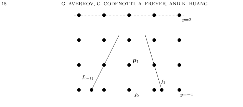
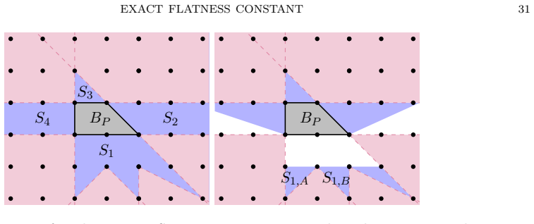
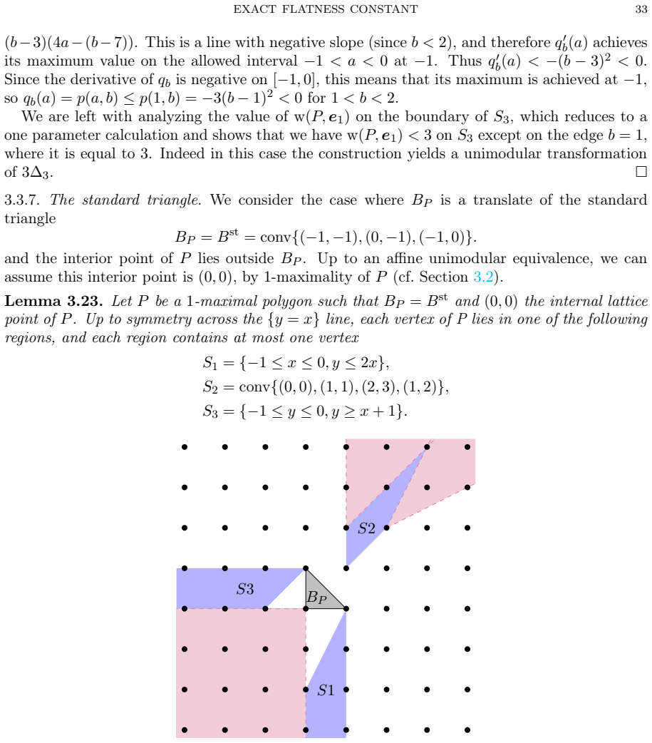
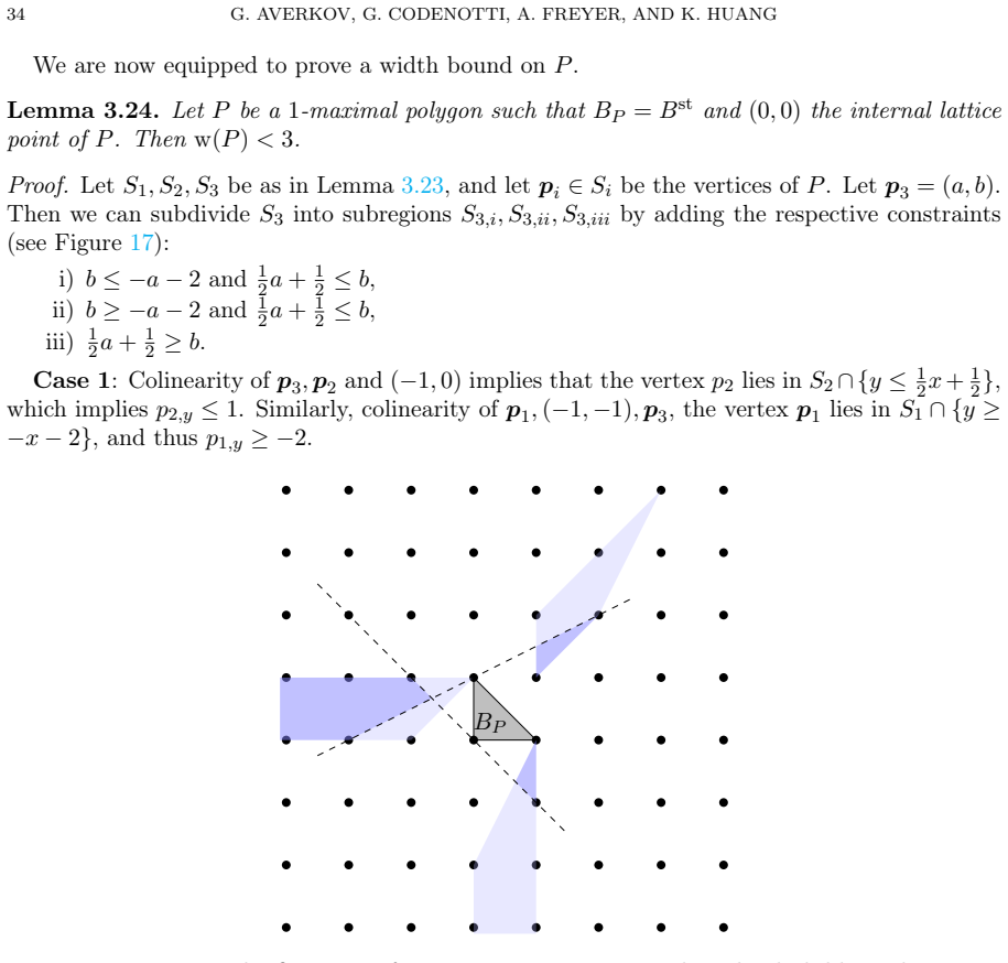
Figures reproduced from arXiv: 2604.27260 by Ansgar Freyer, Gennadiy Averkov, Giulia Codenotti, Kyle Huang.

Figure 1
Figure 1. Figure 1: The edges f(−1) and f1, emanating from f0. As they separate the points (−1, 0),(1, 0) from P, respectively, we see that w(P, e1) = ℓ0. To prove Theorem 1.1 we want to show, for each possible lattice polytope B in the classification of Proposition 3.6, that all polytopes P with blocking polytope BP = B satisfy w(P) ≤ 3. We will now see that Lemma 3.7 allows us to take care of all but finitely many cases, co… view at source ↗
Figure 2
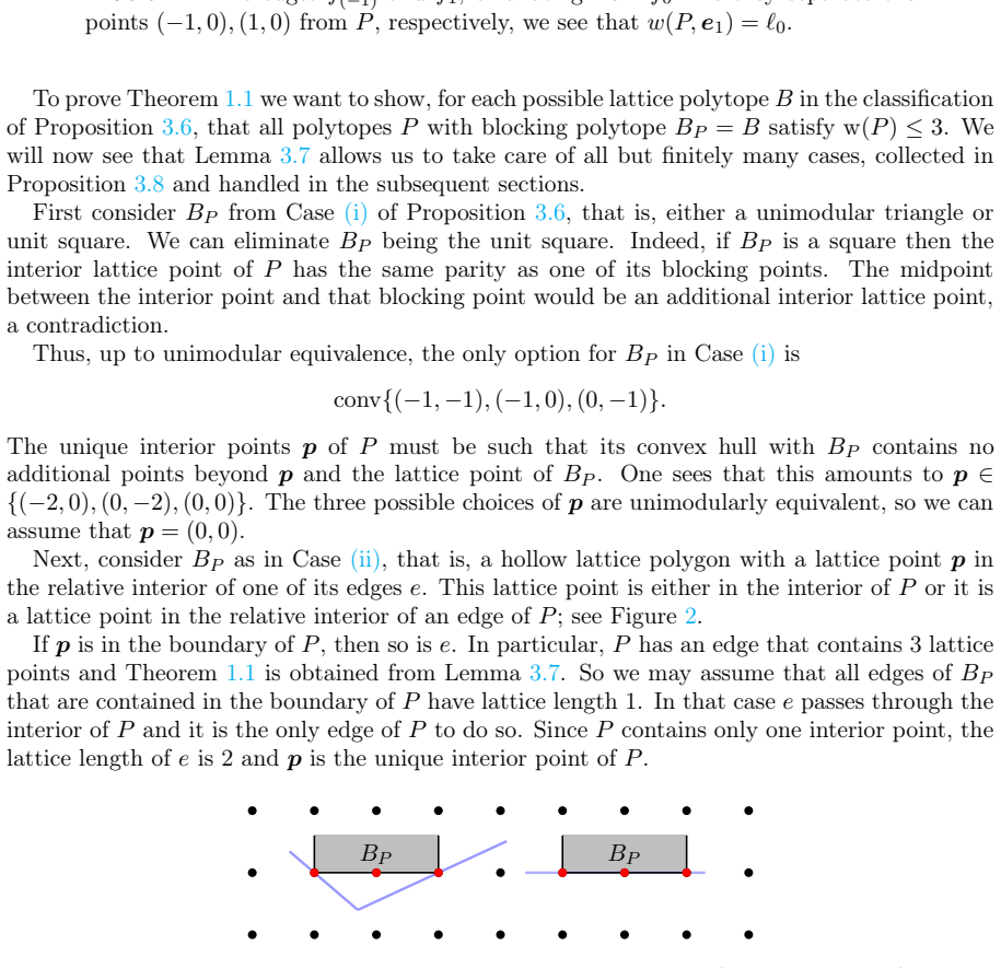
Figure 2. Figure 2: When BP has three colinear boundary points (visualized in red), either the inside point is an interior lattice point of P, as on the left, or all three points lie on an edge of P, as on the right. In this situation Lemma 3.7 applies view at source ↗
Figure 3
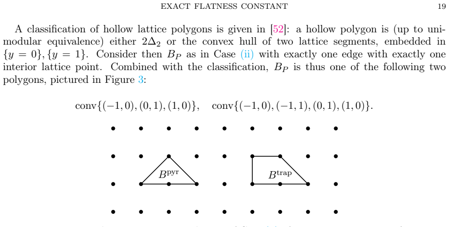
Figure 3. Figure 3: The two remaining polygons of Case (ii) of Proposition 3.6. We refer to them as Bpyr and Btrap, respectively. Now consider BP as in Case (iii). There are 16 lattice polygons (up to unimodular transfor￾mation) with one interior lattice point, see [52]. By Lemma 3.7, we can assume that BP has no edge of lattice length greater than 1. Filtering the list of the 16 so accordingly yields the following 5 polygons… view at source ↗
Figure 4
Figure 4. Figure 4: The 5 remaining polygons of Case (iii) of Proposition 3.6. We refer to them as Bterm, Bkite , Bcross , Bpent , and Bhex, respectively. Compare with view at source ↗
Figure 5
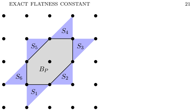
Figure 5. Figure 5: The configuration as in Lemma 3.9. The regions S1, ..., S6 are as labeled, in blue. Observe that the points p1 , p6 must lie between the lines {y − x = −1} and {y − x = 1}, and that p1 , p6 and (−1, −1) are colinear: that is, there exists λ ≥ 0 such that p1 , p6 lie on the line {y + 1 = −λ(x + 1)}. We then see that p1,y + p6,x is minimized if p1 , p6 lie respectively on lines {y − x = −1}, {y − x = 1}, in … view at source ↗
Figure 6
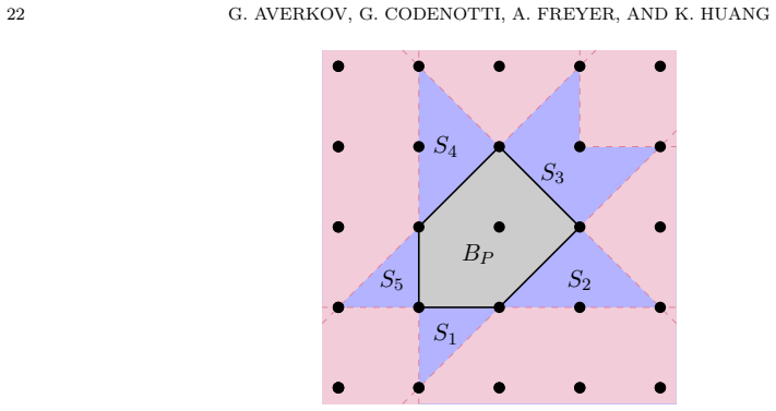
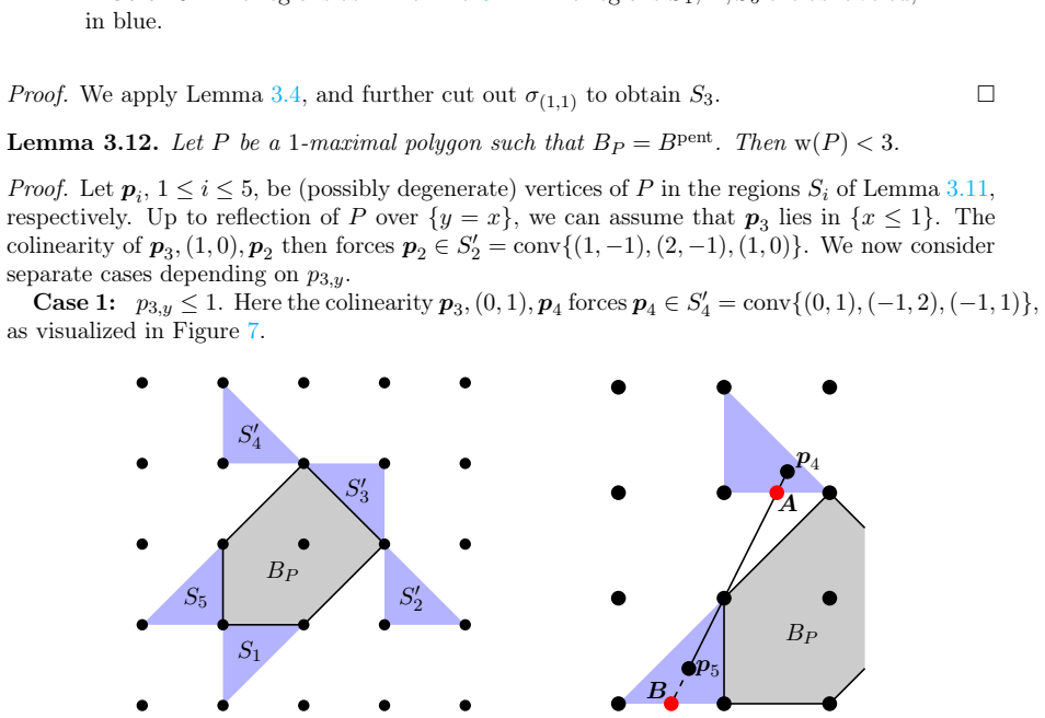
Figure 6. Figure 6: The regions as in Lemma 3.11. The regions S1, ..., S5 are as labeled, in blue. Proof. We apply Lemma 3.4, and further cut out σ(1,1) to obtain S3. □ Lemma 3.12. Let P be a 1-maximal polygon such that BP = Bpent. Then w(P) < 3. Proof. Let pi , 1 ≤ i ≤ 5, be (possibly degenerate) vertices of P in the regions Si of Lemma 3.11, respectively. Up to reflection of P over {y = x}, we can assume that p3 lies in {x … view at source ↗
Figure 7
Figure 7. Figure 7: The regions as in Case 1 of Lemma 3.12. On the right we visualize the points A, B which help relate p4,y and p5,x. We consider now the width of P in directions e1, e2. We have w(P, e1) = p2,x − p5,x, w(P, e2) = p4,y − p1,y. Let L denote the line given by p5 ,(−1, 0), p4 , which are colinear by construction, and let A = L ∩ {y = 1}, B = L ∩ {y = −1}, as in view at source ↗
Figure 8
Figure 8. Figure 8: The regions as in Case 2 of Lemma 3.12. Arguing analogously to case 1, colinearity of p1 ,(−1, −1) and p5 yields p1,y + p5,x ≥ −3, while colinearity p2 ,(1, 0) and p3 yields p2,x + p3,y ≤ 3. Putting these together we obtain w(P, e1) + w(P, e2) = p2,x − p5,x + p3,y − p1,y ≤ 6. Just as in case 1, equality w(P) = 3 can occur only if p3 , p5 lie on {y = x+ 1}, p2 on {y = 2}, and p1 on {y = x − 1}. The only way… view at source ↗
Figure 9
Figure 9. Figure 9: The regions as in Lemma 3.13. Proof. These regions arise by combining Lemma 3.4 and Lemma 3.5 applied to the points (1, 1),(−1, 1),(1, −1), and (−1, −1). □ Lemma 3.14. Let P be a 1-maximal polygon such that BP = Bcross . Then w(P) < 3. Proof. Let p1 , p2 , p3 , p4 be (possibly degenerate) vertices of P in S1, S2, S3, S4, respectively. We first handle some degenerate cases. Claim. If any pi is on the bounda… view at source ↗
Figure 10
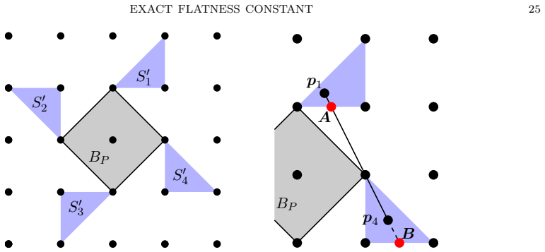
Figure 10. Figure 10: The regions that the vertices of P can lie in. On the right we visualize the points A, B. Let L be the line through the colinear points p4 ,(1, 0), p1 , and let A be the intersection point L ∩ {y = 1} and B be the intersection point L ∩ {y = −1}; see view at source ↗
Figure 11
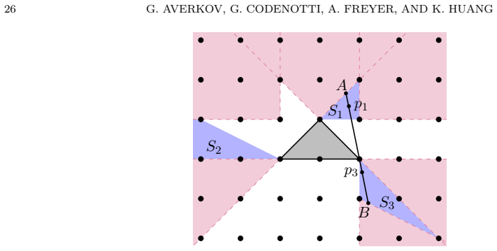
Figure 11. Figure 11: Constraints on P circumscribing BP where BP is the long triangle. The shaded purple regions are open, pointed cones σq for various lattice points q, see Lemma 3.5. By our discussion, we can assume that the vertices of P lie in the shaded blue regions. w(P, e2) = p1,y − p3,y ≤ Ax − Bx. If A = (a, a + 1), with 0 ≤ a ≤ 1, we have B = ( a+3 3a+1 , −2(a+1) 3a+1 ). Thus we can estimate w(P, e2) ≤ 3 (a + 1)2 3a … view at source ↗
Figure 12
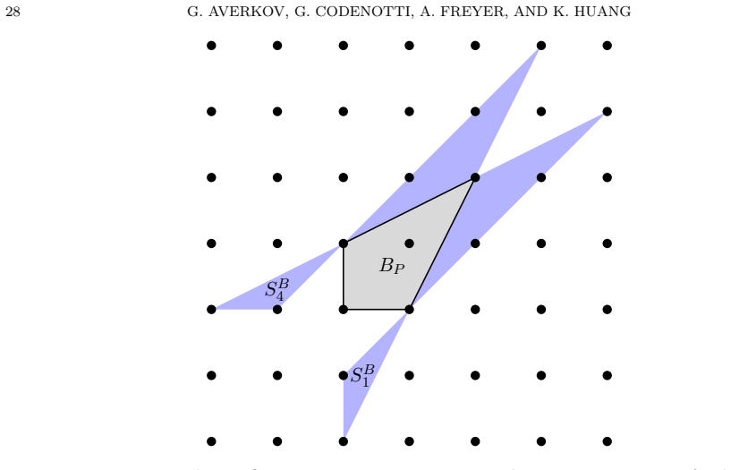
Figure 12. Figure 12: The regions as described in Lemma 3.16. Lemma 3.17. Let P such that BP = Bkite. Then we cannot have p1 ∈ S A 1 \ [(−1, 0),(−2, −1)] and p4 ∈ S A 4 \ [(0, −1),(−1, −2)]. Proof. Towards a contradiction, let p1 , p4 be as described and let p2 , p3 be the vertices of P in S2, S3, respectively. Then by colinearity of p1 ,(0, −1), and p2 and considering the region S2, we see that p2 ∈ conv{(0, −1),(1, −1),(1, 0… view at source ↗
Figure 13
Figure 13. Figure 13: The configuration as in Lemma 3.18. The vertices p2 , p3 are further constrained (compare with S2, S3 of view at source ↗
Figure 14
Figure 14. Figure 14: The regions as in Lemma 3.19. For the width directions e1, e2, e1 − e2, they are realized by vertices of fixed regions. Suppose first that a + 3b = 5. The line {x + 3y = 5} intersects the boundary of the region S2 in the points ( 7 5 , 6 5 ) and (2, 1). For λ ∈ [0, 1], let p2 (λ) = λ(2, 1) + (1 − λ)( 7 5 , 6 5 ). Moreover, let pe3 (λ) ∈ S3 be the intersection point of the line {x = −1} with the line gener… view at source ↗
Figure 15
Figure 15. Figure 15: Left: The regions Si as in Lemma 3.21. Right: The regions can be further constrained by consider the width in direction e2. p3 p1 L3 R3 L ′ 1 R ′ 1 Proof. We denote by p1 , p2 , p3 , p4 the possibly degenerate vertices in the regions S1, S2, S3, S4. Observe that, once we choose p1 and p3 inside their respective regions, we have completely determined the polygon P thanks to the colinearity conditions betwe… view at source ↗
Figure 16
Figure 16. Figure 16: The regions as described in Lemma 3.23. Proof. Since 0 ∈/ BP , there exists an edge e of BP such that 0 ∈ int(Se) (see Section 3.1). Within Se there is a vertex pe of P and we may assume that pe is above the line {y = x}. Since 0 ∈ intP, we have 0 ∈ int(conv(e ∪ {pe})). This implies that pe ∈ σ0 = R 2 >0 (cf. Section 3.1). Lemma 3.5 applied to the open cones σ(1,1), σ(0,1) yields the region S2 from view at source ↗
Figure 17
Figure 17. Figure 17: The first case of Lemma 3.24 is represented as the dark blue sub￾region on the left. Thus w(P, e2) ≤ 3. For equality to hold we would require p1 = (0, −1) and p2 = (1, 1) (see view at source ↗
Figure 18
Figure 18. Figure 18: When w(P, e1) > 3, we can slide p2 to find a P ′ (the dashed triangle) such that w(P ′ , e1 − e2) ≥ w(P, e1 − e2) p ′ 2 , p ′ 1 of P ′ are completely determined by the vertex p3 , by w(P ′ , e1) = 3 and the colinearites given by Bst as the inscribed polygon. Their precise coordinates are p ′ 2 = (a + 3, b + 3b a + 1 ), p ′ 1 = ((b + 1)(a + 3) b − 2 , −1 + (b + 1)(ab + a + 4b + 1) (a + 1)(b − 2) ). Thus, w… view at source ↗
Figure 19
Figure 19. Figure 19: Considering the colinearity restrictions of the vertices of P further restricts the regions its vertices can lie in. There is a cyclic group of affine unimodular transformations cycling the vertices of Bterm. We can write a generator of this group of symmetries as the linear transformation given by σ =  0 −1 1 −1  , σ3 = I. Moreover, the symmetry σ is transitive on the width directions from A, i.e., (3.… view at source ↗
Figure 20
Figure 20. Figure 20: Constructing a perturbation P ′ of P such that the width in direction e2 increases. The polytope P ′ = conv{p ′ 1 , p ′ 2 , p3} is a perturbation of P, it is still a 1-maximal polygon with BP′ = Bterm and its width in direction e2 is larger than that of P, since p1 is a non-trivial convex combination of p ′ 1 , q2 . As we have strict inequalities w(P, e2) < w(P, e1), w(P, e2) < w(P, e1 − e2), and widths a… view at source ↗
Figure 21
Figure 21. Figure 21: Parametrizing circumscribers of Bterm for which the width is at￾tained in directions e1, e2. The lattice Z 2 is shifted by (u, v). need the following colinearity constraints for 1 ≤ i ≤ 3 (here we understand the indices as being modulo 3) fi(x, y, u, v, t) = det    pei qei−1 pei+1 1 1 1    = 0. Further, we have required t ≤ w(P , e e1 − e2) = 2t − x − y. To prove Lemma 3.29 we are thus interested in… view at source ↗
read the original abstract

A variant of the flatness problem from integer programming is studied, in which one considers convex bodies in $\mathbb{R}^d$ with at most $k$ interior lattice points. The maximum lattice width of such a body is denoted by Flt(d,k) and it is related to the classical flatness constant as well as a conjectural dual version of Minkowski's convex body theorem due to Makai. Moreover, it is shown that Flt(2, 1) = 3, i.e., any planar convex body with at most one interior point has lattice width at most three. This leads to an isominwidth inequality for the lattice point enumerator of planar convex bodies.

Editorial analysis

A structured set of objections, weighed in public.

Desk editor's note, referee report, simulated authors' rebuttal, and a circularity audit. Tearing a paper down is the easy half of reading it; the pith above is the substance, this is the friction.

Referee Report

1 major / 0 minor

Summary. The manuscript studies a variant of the flatness problem in which convex bodies in R^d have at most k interior lattice points. It defines Flt(d,k) as the maximum lattice width of such bodies, relates the quantity to the classical flatness constant and to a conjectural dual form of Minkowski's theorem due to Makai, and claims to prove that Flt(2,1)=3. The latter statement is said to imply an isominwidth inequality for the lattice-point enumerator of planar convex bodies.

Significance. If the claimed equality Flt(2,1)=3 holds, the result would supply an exact value for this variant of the flatness constant in the planar one-interior-point case and would furnish a concrete isominwidth inequality, both of which are of interest in discrete convex geometry and integer programming.

major comments (1)
  1. [Abstract] Abstract: the central claim Flt(2,1)=3 is asserted, yet the manuscript consists solely of the abstract and supplies neither the definition of lattice width used, the proof strategy, nor any supporting derivation or example; consequently the load-bearing equality cannot be checked for correctness.

Simulated Author's Rebuttal

1 responses · 1 unresolved

We thank the referee for the comments. We address the single major comment below.

read point-by-point responses
  1. Referee: [Abstract] Abstract: the central claim Flt(2,1)=3 is asserted, yet the manuscript consists solely of the abstract and supplies neither the definition of lattice width used, the proof strategy, nor any supporting derivation or example; consequently the load-bearing equality cannot be checked for correctness.

    Authors: The observation is accurate: the text supplied for review consists solely of the abstract and contains neither the definition of lattice width, the proof strategy, nor any derivation or example. The full manuscript (not available in the present review materials) contains these elements and establishes that every planar convex body with at most one interior lattice point has lattice width at most three. We will resubmit the complete manuscript containing the full argument. revision: yes

standing simulated objections not resolved
  • The explicit definition of lattice width, the proof strategy, and the supporting derivations establishing Flt(2,1)=3, none of which appear in the available manuscript text.

Circularity Check

0 steps flagged

No circularity detected; abstract presents direct claim without inspectable reductions

full rationale

Only the abstract is available, which states that Flt(2,1)=3 is shown for planar convex bodies with at most one interior lattice point and relates it to the flatness problem and Makai's conjecture. No equations, derivations, self-citations, fitted parameters, or ansatzes are provided that could reduce the result to its inputs by construction. The claim is framed as a direct proof, making the derivation self-contained against external benchmarks with no load-bearing circular steps identifiable.

Axiom & Free-Parameter Ledger

0 free parameters · 1 axioms · 0 invented entities

Abstract-only review supplies no explicit free parameters, invented entities, or non-standard axioms; the setup relies on the conventional definitions of convex bodies, lattice width, and interior lattice points in R^d.

axioms (1)
  • domain assumption Standard definition of lattice width and interior lattice points for convex bodies in R^d
    The variant of the flatness problem and the quantity Flt(d,k) are defined using these background notions.

pith-pipeline@v0.9.1-grok · 5633 in / 1190 out tokens · 44565 ms · 2026-07-01T08:18:28.339556+00:00 · methodology

discussion (0)

Sign in with ORCID, Apple, or X to comment. Anyone can read and Pith papers without signing in.