Scalar Field Estimation with Mobile Sensor Networks
Pith reviewed 2026-05-25 11:01 UTC · model grok-4.3
The pith
Mobile sensors estimate a scalar field exactly when their paths satisfy persistence-like conditions on the measurements.
A machine-rendered reading of the paper's core claim, the machinery that carries it, and where it could break.
Core claim
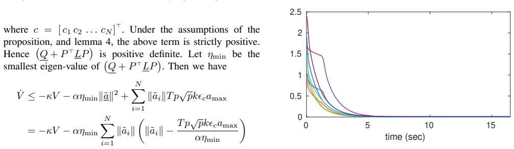
For a scalar field that can be expressed exactly as a finite sum of positive definite radial basis kernels with known centers and shapes, the parameter vector estimated from instantaneous point measurements by mobile sensors converges asymptotically to the true parameter vector whenever the collective sensor trajectories satisfy persistence-like conditions; the proof proceeds by constructing an adaptive estimator whose stability is shown via a Lyapunov function whose derivative is made negative semi-definite under those motion constraints.
What carries the argument
Persistence-like conditions on the collective trajectories of the mobile sensors, which ensure that the regressor matrix formed by the radial basis evaluations remains sufficiently exciting for the adaptive parameter update law.
If this is right
- Parameter estimates converge to their true values under the designed motion.
- The closed-loop estimator remains stable in the Lyapunov sense.
- Sensor paths can be generated without prior knowledge of the field values.
- The same framework applies to any finite network of mobile sensors that can be steered to meet the excitation conditions.
Where Pith is reading between the lines
- The same persistence-based motion planning could be tested on fields that are only approximately representable by radial basis kernels, with the resulting error bounds derived from the approximation residual.
- The method suggests a separation between path planning (done without field knowledge) and online parameter adaptation that might be useful for other distributed sensing tasks such as gradient field reconstruction.
- If the radial basis centers are allowed to be adapted as well, the persistence conditions would need to be strengthened to guarantee joint convergence of both centers and weights.
Load-bearing premise
The scalar field must be exactly equal to a finite sum of positive definite radial basis kernels whose centers and shapes are known before any measurements are taken.
What would settle it
A counter-example in which sensors follow trajectories that satisfy the stated persistence conditions yet the parameter estimates fail to converge when the true field deviates from the assumed radial-basis representation.
Figures


read the original abstract
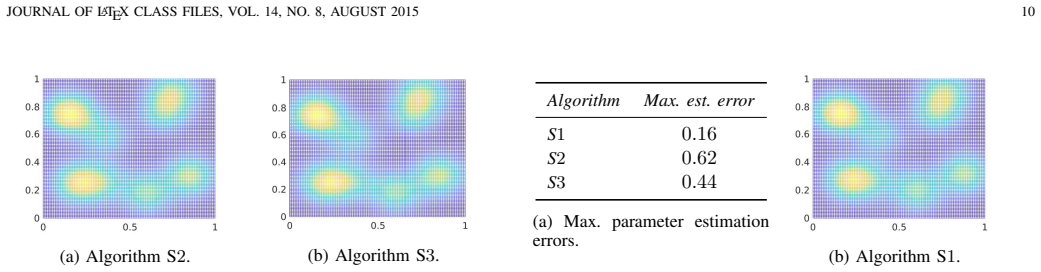
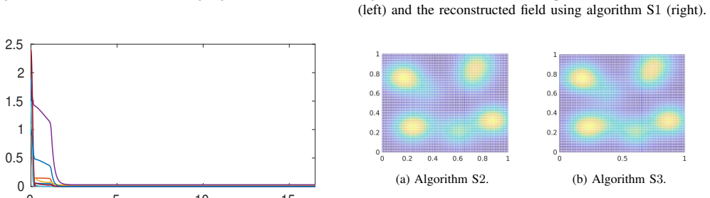
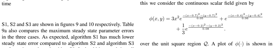
In this paper, we consider the problem of estimating a scalar field using a network of mobile sensors which can measure the value of the field at their instantaneous location. The scalar field to be estimated is assumed to be represented by positive definite radial basis kernels and we use techniques from adaptive control and Lyapunov analysis to prove the stability of the proposed estimation algorithm. The convergence of the estimated parameter values to the true values is guaranteed by planning the motion of the mobile sensors to satisfy persistence-like conditions.
Editorial analysis
A structured set of objections, weighed in public.
Referee Report
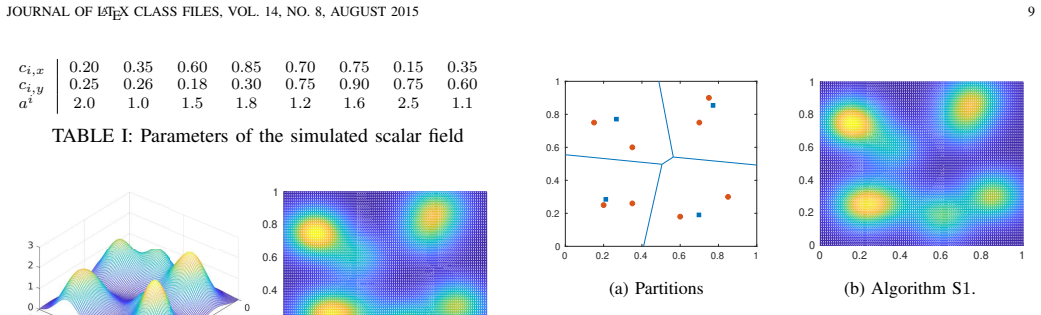
Summary. The paper considers estimating a scalar field using mobile sensors that measure the field at their locations. The field is modeled as a finite sum of positive definite radial basis kernels with a priori known centers and shapes. An adaptive estimation scheme is proposed whose stability is proved via Lyapunov analysis drawn from adaptive control. Parameter estimates are shown to converge to their true values provided the sensors' trajectories are planned to satisfy persistence-like excitation conditions.
Significance. If the central claims hold, the work supplies a Lyapunov-based guarantee that sensor motion can be designed to enforce parameter convergence for fields exactly spanned by a known finite RBF dictionary. This links adaptive-control persistence conditions directly to trajectory planning and could inform coverage or exploration strategies in environmental monitoring. The approach is parameter-free in the sense that the regressor structure is fixed before deployment, which is a positive feature when the modeling assumption is satisfied.
major comments (2)
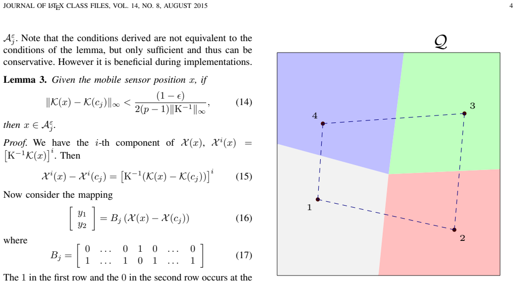
- [Abstract / Problem Formulation] Abstract and problem statement: the claim that estimated parameters converge to the 'true values' is load-bearing on the modeling assumption that the scalar field lies exactly in the finite-dimensional span of the chosen RBFs whose centers and widths are known a priori. If the field contains components outside this span, the Lyapunov argument only establishes convergence to the orthogonal projection onto that span, not to the claimed true parameters. This distinction must be stated explicitly and the result reframed accordingly.
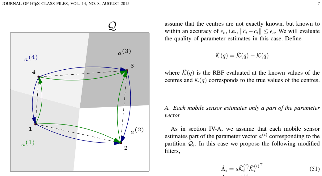
- [Motion Planning / Persistence Conditions] Motion-planning section: the persistence-like conditions must be shown to be satisfiable using only quantities known before deployment (sensor kinematics and the fixed RBF centers), without dependence on the unknown field values or on the running parameter estimates. If the planner uses estimates in a way that can destroy excitation, the convergence guarantee is circular. A concrete verification that the generated trajectories remain persistently exciting independently of the field is required.
minor comments (2)
- [Abstract] Notation for the RBF widths and centers should be introduced once and used consistently; the abstract refers to 'positive definite radial basis kernels' without specifying whether widths are identical or per-kernel.
- [Abstract] The phrase 'persistence-like conditions' should be replaced by a precise reference to the standard persistence-of-excitation definition used in the Lyapunov analysis (e.g., the integral condition on the regressor).
Simulated Author's Rebuttal
We thank the referee for the constructive comments, which help clarify the scope and assumptions of our work. We address each major comment below and will revise the manuscript accordingly.
read point-by-point responses
-
Referee: [Abstract / Problem Formulation] Abstract and problem statement: the claim that estimated parameters converge to the 'true values' is load-bearing on the modeling assumption that the scalar field lies exactly in the finite-dimensional span of the chosen RBFs whose centers and widths are known a priori. If the field contains components outside this span, the Lyapunov argument only establishes convergence to the orthogonal projection onto that span, not to the claimed true parameters. This distinction must be stated explicitly and the result reframed accordingly.
Authors: We agree that the distinction is important for precision. The manuscript explicitly assumes that the scalar field lies exactly in the finite span of the chosen RBFs (see abstract and Section II). Under this assumption, the Lyapunov analysis establishes convergence to the true parameters. If the field has components outside the span, the estimates converge to the orthogonal projection. In the revision we will add an explicit statement of this modeling assumption in the abstract and problem formulation, and reframe the convergence claim to hold under the exact-span assumption (or to the projection otherwise). revision: yes
-
Referee: [Motion Planning / Persistence Conditions] Motion-planning section: the persistence-like conditions must be shown to be satisfiable using only quantities known before deployment (sensor kinematics and the fixed RBF centers), without dependence on the unknown field values or on the running parameter estimates. If the planner uses estimates in a way that can destroy excitation, the convergence guarantee is circular. A concrete verification that the generated trajectories remain persistently exciting independently of the field is required.
Authors: The regressor is formed from sensor positions and the a priori known RBF centers/shapes; the persistence conditions are therefore defined solely in terms of these known quantities and the sensor kinematics. The motion planner is designed to generate trajectories that satisfy the persistence conditions using only these pre-deployment quantities and does not feed back the running parameter estimates in a manner that can destroy excitation. In the revised manuscript we will add a concrete verification (e.g., an explicit trajectory construction or numerical check) demonstrating that the generated paths remain persistently exciting independently of the unknown field values. revision: yes
Circularity Check
No circularity: standard adaptive control + Lyapunov applied to exact RBF span assumption
full rationale
The derivation chain rests on the explicit modeling assumption that the unknown scalar field lies exactly in the finite-dimensional span of a priori known positive-definite RBF kernels, followed by application of classical persistence-of-excitation results from adaptive control theory (external to the paper) and standard Lyapunov analysis to guarantee parameter convergence when sensor trajectories satisfy the PE condition. No step reduces a claimed prediction to a fitted parameter by construction, no self-citation is invoked as a load-bearing uniqueness theorem, and the motion-planning requirement is stated as an independent design task using only known quantities. The central claim therefore remains non-tautological and externally grounded.
Axiom & Free-Parameter Ledger
axioms (2)
- domain assumption The scalar field is exactly representable by a finite linear combination of known positive definite radial basis kernels.
- domain assumption Sensor trajectories can be planned to satisfy persistence-like excitation conditions.
Reference graph
Works this paper leans on
-
[1]
Coordination of groups of mobile autonomous agents using nearest neighbor rules,
A. Jadbabaie and J. Lin, “Coordination of groups of mobile autonomous agents using nearest neighbor rules,” Automatic Control, IEEE Transac- tions on, vol. 48, no. 6, pp. 988–1001, 2003
work page 2003
-
[2]
Recent research in cooperative control of multivehicle systems,
R. M. Murray, “Recent research in cooperative control of multivehicle systems,” Journal of Dynamic Systems, Measurement, and Control , vol. 129, no. 5, pp. 571–583, 2007
work page 2007
-
[3]
Consensus and cooperation in networked multi-agent systems,
R. Olfati-Saber, A. Fax, and R. M. Murray, “Consensus and cooperation in networked multi-agent systems,” Proceedings of the IEEE , vol. 95, no. 1, pp. 215–233, 2007
work page 2007
-
[4]
Flocking in fixed and switching networks,
H. Tanner, A. Jadbabaie, and G. Pappas, “Flocking in fixed and switching networks,” Automatic Control, IEEE Transactions on, vol. 52, no. 5, pp. 863–868, May 2007
work page 2007
-
[5]
Coverage control for mobile sensing networks,
J. Cortes, S. Martinez, T. Karatas, and F. Bullo, “Coverage control for mobile sensing networks,” IEEE Transactions on Automatic Control , vol. 20, no. 2, pp. 243–255, Apr. 2004
work page 2004
-
[6]
Estimating inhomogeneous fields using wireless sensor networks,
R. Nowak, U. Mitra, and R. Willett, “Estimating inhomogeneous fields using wireless sensor networks,” IEEE Journal on Selected Areas in Communications, vol. 22, no. 6, pp. 999–1006, Aug 2004
work page 2004
-
[7]
Matched source-channel commu- nication for field estimation in wireless sensor network,
W. Bajwa, A. Sayeed, and R. Nowak, “Matched source-channel commu- nication for field estimation in wireless sensor network,” in IPSN 2005. Fourth International Symposium on Information Processing in Sensor Networks, 2005., April 2005, pp. 332–339
work page 2005
-
[8]
Static field estimation using a wireless sensor network based on the finite element method,
T. Van Waterschoot and G. Leus, “Static field estimation using a wireless sensor network based on the finite element method,” in 2011 4th IEEE International Workshop on Computational Advances in Multi-Sensor Adaptive Processing (CAMSAP) , Dec 2011, pp. 369–372
work page 2011
-
[9]
Spatio-temporal characteristics of point and field sources in wireless sensor networks,
M. C. Vuran and O. B. Akan, “Spatio-temporal characteristics of point and field sources in wireless sensor networks,” in 2006 IEEE International Conference on Communications , vol. 1, June 2006, pp. 234–239
work page 2006
-
[10]
H. Zhang, J. M. F. Moura, and B. Krogh, “Dynamic field estimation using wireless sensor networks: Tradeoffs between estimation error and communication cost,” IEEE Transactions on Signal Processing, vol. 57, no. 6, pp. 2383–2395, June 2009
work page 2009
-
[11]
D. Dardari, A. Conti, C. Buratti, and R. Verdone, “Mathematical evaluation of environmental monitoring estimation error through energy- efficient wireless sensor networks,” IEEE Transactions on Mobile Com- puting, vol. 6, no. 7, pp. 790–802, July 2007
work page 2007
-
[12]
Distributed estimation and detection for sensor networks using hidden markov random field models,
A. Dogandzic and B. Zhang, “Distributed estimation and detection for sensor networks using hidden markov random field models,” IEEE Transactions on Signal Processing , vol. 54, no. 8, pp. 3200–3215, Aug 2006
work page 2006
-
[13]
Adaptive information collection by robotic sensor networks for spatial estimation,
R. Graham and J. Cortes, “Adaptive information collection by robotic sensor networks for spatial estimation,” IEEE Transactions on Automatic Control, vol. 57, no. 6, pp. 1404–1419, June 2012
work page 2012
-
[14]
Random field reconstruction with quantization in wireless sensor networks,
I. Nevat, G. W. Peters, and I. B. Collings, “Random field reconstruction with quantization in wireless sensor networks,” IEEE Transactions on Signal Processing, vol. 61, no. 23, pp. 6020–6033, Dec 2013
work page 2013
-
[15]
R. K. Ramachandran and S. Berman, “The effect of communication topology on scalar field estimation by large networks with partially accessible measurements,” in 2017 American Control Conference (ACC), May 2017, pp. 3886–3893
work page 2017
-
[16]
Scalar field estimation using adaptive networks,
Y . P. Bergamo and C. G. Lopes, “Scalar field estimation using adaptive networks,” in 2012 IEEE International Conference on Acoustics, Speech and Signal Processing (ICASSP) , March 2012, pp. 3565–3568
work page 2012
-
[17]
Distributed sensor fusion for scalar field map- ping using mobile sensor networks,
H. M. La and W. Sheng, “Distributed sensor fusion for scalar field map- ping using mobile sensor networks,” IEEE Transactions on Cybernetics, vol. 43, no. 2, pp. 766–778, April 2013
work page 2013
-
[18]
Cooperative and active sensing in mobile sensor networks for scalar field mapping,
H. M. La, W. Sheng, and J. Chen, “Cooperative and active sensing in mobile sensor networks for scalar field mapping,” IEEE Transactions on Systems, Man, and Cybernetics: Systems , vol. 45, no. 1, pp. 1–12, Jan 2015
work page 2015
-
[19]
W. Wu and F. Zhang, “Cooperative exploration of level surfaces of three dimensional scalar fields,” Automatica, vol. 47, no. 9, pp. 2044–2051, Sep. 2011. [Online]. Available: http://dx.doi.org/10.1016/j. automatica.2011.06.001
work page doi:10.1016/j 2044
-
[20]
Adaptive sampling for estimating a scalar field using a robotic boat and a sensor network,
B. Zhang and G. S. Sukhatme, “Adaptive sampling for estimating a scalar field using a robotic boat and a sensor network,” in Proceedings 2007 IEEE International Conference on Robotics and Automation, April 2007, pp. 3673–3680
work page 2007
-
[21]
Decentralized, adaptive cover- age control for networked robots,
M. Schwager, D. Rus, and J.-J. Slotine, “Decentralized, adaptive cover- age control for networked robots,” Int. J. Rob. Res. , vol. 28, no. 3, pp. 357–375, Mar. 2009
work page 2009
-
[22]
Decentralized Adaptive Coverage Control of Nonholonomic Mobile Robots,
R. Abdul Razak, S. Srikant, and H. Chung, “Decentralized Adaptive Coverage Control of Nonholonomic Mobile Robots,” in 10th IFAC Symposium on Nonlinear Control Systems , 2016, pp. 1173–1178
work page 2016
-
[23]
Decentralized and adaptive control of multiple nonholonomic robots for sensing coverage,
——, “Decentralized and adaptive control of multiple nonholonomic robots for sensing coverage,” International Journal of Robust and Nonlinear Control , vol. 28, no. 6, pp. 2636–2650, 2018. [Online]. Available: https://onlinelibrary.wiley.com/doi/abs/10.1002/rnc.4041
-
[24]
Distributed coverage control of mobile sensors: Generalized approach using distance functions,
R. A. Razak, S. Srikant, and H. Chung, “Distributed coverage control of mobile sensors: Generalized approach using distance functions,” in 2018 IEEE Conference on Decision and Control (CDC) , Dec 2018, pp. 3323–3328
work page 2018
-
[25]
Universal approximation using radial-basis- function networks,
J. Park and I. W. Sandberg, “Universal approximation using radial-basis- function networks,” Neural Computation , vol. 3, no. 2, pp. 246–257, June 1991
work page 1991
- [26]
-
[27]
Interpolation of scattered data: distance matrices and conditionally positive definite functions,
C. Micchelli, “Interpolation of scattered data: distance matrices and conditionally positive definite functions,” Constr. Approx., vol. 2, pp. 11–22, 1986
work page 1986
-
[28]
D. Gorinevsky, “On the persistency of excitation in radial basis function network identification of nonlinear systems,” IEEE Transactions on Neural Networks, vol. 6, no. 5, pp. 1237–1244, 1995
work page 1995
-
[29]
M. Mesbahi and M. Egerstedt, Graph theoretic methods in multiagent networks. Princeton University Press, 2010, vol. 33
work page 2010
discussion (0)
Sign in with ORCID, Apple, or X to comment. Anyone can read and Pith papers without signing in.