Topology-Aware 3D Gaussian Splatting: Leveraging Persistent Homology for Optimized Structural Integrity

Jiaqi Feng; Ning An; Shaohua Liu; Tianqi Shen; Ziye Ma

REVIEW 4 major objections 6 minor 13 references

Topology-Aware 3D Gaussian Splatting: Leveraging Persistent Homology for Optimized Structural Integrity

T0 review · 4 major / 6 minor · reviewed 2026-08-11 · deepseek-v4-flash

Challenge this review Re-run · record.json Download PDF Read on arXiv ↗ Review JSON

Pith's one-line read Topology-GS inserts persistent homology in two places—densifying the initial point cloud and regularizing training—and reports better PSNR, SSIM, and LPIPS than earlier splatting methods.

desk verdict A solid empirical TDA-for-3DGS paper whose abstract overclaims LPIPS, with a convergence theorem that is more imported than proven; send it to review and make them fix the claim. read the letter →

arxiv 2412.16619 v4 pith:546FNKNF submitted 2024-12-21 cs.CV cs.LGeess.IVmath.ATmath.GT

Tianqi Shen , Shaohua Liu , Jiaqi Feng , Ziye Ma , Ning An This is my paper · ORCID

classification cs.CVcs.LGeess.IVmath.ATmath.GT

keywords 3DGaussianSplattingpersistenthomologynovel-viewsynthesispointclouddensificationVoronoiinterpolationtopologicallossperceptualsimilarityconvergenceguarantee

verification ladder T0 review T1 audit T2 compute T3 formal

The pith

A machine-rendered reading of the paper's core claim, the machinery that carries it, and where it could break.

The reading

The paper sets out to show that persistent homology—the study of when loops, holes, and connected components are born and die as a shape grows—can fix two known weaknesses of 3D Gaussian Splatting (3D-GS), the point-based rendering method for novel-view synthesis. Sparse Structure-from-Motion point clouds under-cover low-curvature surfaces, so the paper introduces Local Persistent Voronoi Interpolation (LPVI): before training it densifies the cloud locally, using the Wasserstein distance between persistence diagrams as a topological-difference check that decides whether safe 3D interpolation is possible or the algorithm must fall back to interpolation on a 2D plane. During optimization, PersLoss—a differentiable regularizer comparing the longest-lived topological features (truncated persistence barcodes) of the rendered and ground-truth images, seen as point clouds in RGB space—is switched on only during the adaptive density-control stage. On the Mip-NeRF360, Tanks & Temples, and Deep Blending benchmarks, Topology-GS reports higher PSNR and SSIM than every compared method on all three datasets and the lowest LPIPS on two of them, with minor memory cost and no inference-time cost. A reader should care because the paper demonstrates a structural prior that needs no extra neural network, comes with a stated convergence guarantee for the combined loss, and targets exactly the perceptual gap that pixel-level metrics miss.

What carries the argument

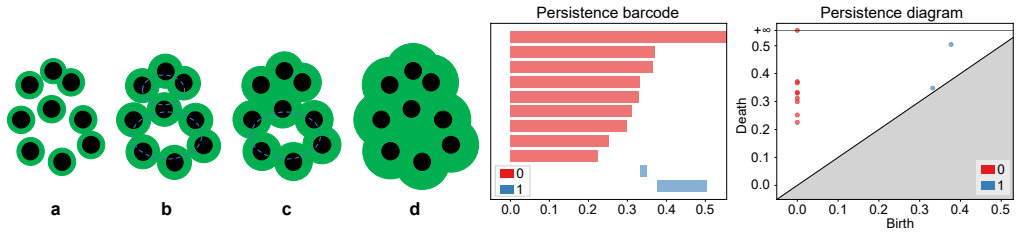
The machinery is persistent homology over $\alpha$ complexes of point sets, packaged as persistence barcodes: as a filtration radius $\alpha$ grows, each connected component, loop, or void records an interval from birth to death, and longer intervals mark features the authors treat as structurally significant. LPVI uses the Wasserstein distance between two local persistence diagrams as its TopoDiff gate, deciding when adding 3D Voronoi vertices is topologically safe versus when to switch to 2D-plane interpolation. PersLoss uses the truncated top-$k$ barcodes of the rendered and ground-truth images reshaped into RGB point clouds, matched by sorted lifespan, and turns the birth–death coordinate differences into a differentiable loss. The convergence theorem binds the two uses: with $B = k_0 + k_1 + k_2$ kept small, the sorted matching with no shrinking-cost regularizer is assumed to approximate the Wasserstein-optimal topological loss, and the step-size bound $\eta \le \min\left\{\frac{1}{2\ell_2 + 10\lambda_{\mathrm{topo}}B},\ \frac{\epsilon}{4096\lambda_{\mathrm{topo}}^2 B^2}\right\}$ yields termination in $O(1/\epsilon)$ iterations.

What would settle it

Render a test scene with dense true topology, such as a chain-link fence whose many loops have nearly equal lifespans, and train Topology-GS while increasing the truncation counts $k_0$, $k_1$, $k_2$: the paper's own convergence bound tightens as $1/B^2$ for $B = k_0+k_1+k_2$, so a fixed learning rate should eventually diverge, and if instead quality keeps improving, the assumption that sorted-lifespan matching approximates the exact Wasserstein distance (the paper's Assumptions A1–A2) is doing more work than the analysis accounts for.

Watch

Extended reading notes

Core claim

The central claim is that one mathematical tool—persistent homology—can be used at two moments of the 3D-GS pipeline to restore structural integrity at two levels. At initialization, LPVI looks at each point of the sparse SfM cloud with its $K$ nearest neighbors, computes the persistence diagrams of that local set before and after adding Voronoi-tessellation vertices, and accepts the 3D interpolation only when the Wasserstein distance between the two diagrams stays below a threshold $\tau$; otherwise it interpolates on a PCA-fitted plane and maps the new points back, a choice the authors justify by the manifold hypothesis for low-curvature regions. During optimization, PersLoss reshapes the rendered and ground-truth images into $HW \times 3$ RGB point clouds, computes their $\alpha$-complex persistence barcodes, keeps the $k_0$, $k_1$, and $k_2$ longest-lived features in homology dimensions 0, 1, and 2, matches them by sorted lifespan rather than by optimal assignment, and penalizes the squared birth and death differences weighted by Betti numbers. The paper proves that this topology-aware total loss—PersLoss plus the usual L1 and SSIM supervision—terminates in $O(1/\epsilon)$ iterations under regularity assumptions on the filter function and the supervision loss, provided the step size obeys the bound in Theorem 1, and that the small truncation count $B = k_0 + k_1 + k_2$ is what keeps that bound practical. The empirical statement is that Topology-GS achieves state-of-the-art PSNR, SSIM, and LPIPS on the three benchmarks, which the authors read as the first successful integration of topology into 3D-GS.

Load-bearing premise

The load-bearing premise is that the few longest-lived topological features of the rendered and ground-truth images, matched by rank instead of by true geometric correspondence, give a faithful enough measure of perceptual difference that shrinking that measure during training improves rendering the way the paper claims; the paper asserts this as Assumptions A1 and A2 in the appendix rather than deriving or testing it.

Editorial extensions

If this is right

On the three reported benchmarks, Topology-GS tops every compared method in PSNR and SSIM and lowers LPIPS relative to the Scaffold-GS baseline on every dataset, so adopting it gives both sharper pixels and closer perceptual features.
PersLoss runs only during the adaptive density-control stage of training, so the perceptual gains come with no added inference cost and only a small training-time and memory overhead (under 20 MB per scene from LPVI).
The depth-map comparisons show LPVI smooths depth in low-curvature regions while PersLoss sharpens depth at structural boundaries, indicating that the topological constraints improve geometry rather than pixel statistics alone.
The ablations show the two contributions are nearly separable—LPVI carries the PSNR and SSIM gains while PersLoss carries the LPIPS gains—so each can be adopted independently depending on which deficiency matters.
Theorem 1 licenses using PersLoss together with L1 and SSIM supervision and the adaptive density control without a separate shrinking-cost regularizer, so the extra topological term does not require reworking the 3D-GS optimization loop.

Reading between the lines

Editorial extensions of the paper, not claims the author makes directly.

Editorial inference: the 'outperforms earlier work' summary is an average statement; the paper's own Table 1 shows Pixel-GS still reports the lower LPIPS on Mip-NeRF360 (0.165 versus 0.179), so the safest public reading is best on average across benchmarks rather than best in every cell.
Extension: the TopoDiff gate is not specific to Voronoi interpolation—the same local persistence-diagram distance could guard any densification, pruning, or smoothing step in a point-cloud pipeline, making persistent homology a generic topology-safety check.
Testable variant: computing PersLoss on other filter functions (grayscale intensity, depth, or the feature maps of a pretrained network) instead of raw RGB coordinates would reveal whether the reported gains come from color-distribution topology or spatial-structure topology, and would show how closely the loss tracks what LPIPS actually measures.
Design implication: the truncation counts $k_0$, $k_1$, $k_2$ are the method's real tuning dials—too few retained features and PersLoss misses structure, too many and the step-size bound collapses as $1/B^2$ while noise bars dominate, exactly the trade-off the paper's Figure 8 and its appendix remark about $B$ describe.

Share X Bluesky LinkedIn Reddit HN

Signed reviews

No signed human review yet.

Editorial analysis

A structured set of objections, weighed in public.

Desk editor's note, referee report, and a circularity audit.

Desk Editor's Note

read the letter

Read this one for the empirical package, not the theory. The contribution is a plausible combination: LPVI, a persistent-homology-guided Voronoi interpolation for the initial sparse point cloud, and PersLoss, a barcode-matching regularizer activated during the ADC stage. The ablations in Table 2 support both components, and Table 1 shows modest but consistent PSNR/SSIM gains over Scaffold-GS, plus a small LPIPS win on Tanks & Temples and Deep Blending. That is a legitimate result for the 3DGS subfield, and the TDA hook is new relative to prior PH-in-point-cloud work.

Now the soft spots.

First, the abstract overclaims LPIPS. The paper says it outperforms existing methods in PSNR, SSIM, and LPIPS, but Table 1 contradicts that on Mip-NeRF360: Pixel-GS reports 0.165, Topology-GS 0.179. On the three-dataset average, Pixel-GS also wins. That is not subtle. The experiments section's claim of a 'substantial reduction in LPIPS across all datasets' is also not supported; the reduction is relative to their baseline, not to all methods. They need to fix the claim or report per-scene numbers.

Second, the convergence theorem is imported from Zhang et al. 2022 and rests on assumptions A1 and A2 that the paper asserts rather than defends. A1 sets Lreg = 0, justified by truncation; A2 says PersLoss is bounded above by the Wasserstein distance, justified by 'negligible' error between length-based matching and optimal matching. The paper does not test that empirically, and the truncation is the very thing being optimized, so the chain from relaxed loss to the actual rendered-image loss is weak. I would treat Theorem 1 as a borrowed guarantee for a neighboring problem, not a guarantee for this pipeline. That is more framing than fatal, since the empirical result does not depend on the theorem, but the authors should not present it as their own convergence proof.

Third, reproducibility: the code link is there but no commit hash, and 'each scene run once on each of eight GPUs and averaged' is not the same as per-scene statistics; no error bars are given. Minor.

Overall, the central argument that the combination helps holds up at the level of Table 1 and the ablations. The paper is for researchers working on 3DGS densification and TDA-based losses in rendering, and it deserves a serious referee—the method is clearly described and the ablations are honest enough to fix. I would send it to review, asking for a corrected LPIPS claim, per-scene numbers, and a softened theory section.

Referee Report

4 major / 6 minor

Summary. The paper proposes Topology-GS, a 3D Gaussian Splatting variant with two novel components: LPVI, a persistent-homology-guided interpolation step that densifies sparse SfM point clouds while adaptively switching between 3D and 2D Voronoi interpolation based on a topological-difference threshold, and PersLoss, a regularization term that compares truncated persistence barcodes of rendered and ground-truth images. The method is evaluated on Mip-NeRF360, Tanks & Temples, and Deep Blending, with ablations, hyperparameter sensitivity studies, and extended experiments on NeRF Synthetic, BungeeNeRF, and IMW2020. The paper claims state-of-the-art PSNR, SSIM, and LPIPS, and provides an appendix with a convergence theorem for the topology-aware total loss, adapted from Zhang et al. (2022).

Significance. If the reported improvements hold, the paper would make a useful contribution: applying persistent homology to Gaussian Splatting for both initialization densification and training-time regularization is a plausible and relatively unexplored direction. The authors ship code, report abundant quantitative results, include ablations for each component, and test across multiple benchmark families. These are concrete strengths. However, the headline LPIPS claim is contradicted by the paper's own Table 1, and the theoretical convergence guarantee rests on assumptions about the relationship between PersLoss and the Wasserstein distance that are asserted rather than established. The PSNR and SSIM claims appear supportable, but the central 'outperforms existing methods in terms of PSNR, SSIM, and LPIPS' statement needs to be corrected or substantially qualified before the paper can be recommended for publication.

major comments (4)

[Abstract; Experiments, Overall Rendering Quality; Table 1] The abstract and the 'Overall Rendering Quality' subsection claim that Topology-GS outperforms existing methods in LPIPS and that PersLoss leads to a substantial LPIPS reduction across all datasets. Table 1 contradicts this. Pixel-GS reports LPIPS 0.165 on Mip-NeRF360, 0.161 on Tanks & Temples, and 0.251 on Deep Blending; Topology-GS reports 0.179, 0.160, and 0.245. The unweighted three-dataset averages are 0.1923 for Pixel-GS versus 0.1947 for Topology-GS, and a dataset-size-weighted average (7:2:2) gives 0.1799 versus 0.1875. Thus the unqualified LPIPS-superiority claim is false as written. The PSNR and SSIM claims may survive, but the LPIPS claim must be removed or qualified (e.g., 'lower LPIPS than Scaffold-GS on all three datasets').
[Appendix B3-B4; Assumptions A1-A2] The convergence theorem in Appendix C rests on Assumption A1 (Lreg = 0) and Assumption A2 (PersLoss ≤ d2(Dgm(f), Dgm(g))). Both are asserted rather than derived. A2 is particularly hard to justify: PersLoss matches truncated top-k barcodes by sorted lifespan, which is not generally an optimal Wasserstein matching, and truncation can omit points that the optimal matching would send to the diagonal. Since the proof of Theorem 1 replaces PersLoss with the optimal-matching loss Ltopo (Definition 1 in B4), this inequality is load-bearing for the claimed convergence guarantee. Please validate A2 empirically on representative rendered/ground-truth image pairs by comparing PersLoss with the exact 2-Wasserstein distance, or state the theorem as conditional on a verified inequality.
[Appendix B5, Eq. (18)] Equation (18) defines the matching as γt = arg max Σ (Bγ(p)^2 + Dγ(p)^2), which maximizes the loss, while Definition 1 in Appendix B4 minimizes the same sum. This sign inconsistency appears in the core derivation and should be corrected; as written it invalidates the derivation of Lemma 3, which is imported from Zhang et al. (2022).
[Main text, Theorem 1; Appendix C1] The quantity B is defined in the main text as B = k0 + k1 + k2, the number of retained barcodes, but in Appendix C1 it is defined as B = card(Dgm*), the cardinality of the full ground-truth diagram excluding the diagonal. These are not the same, and the step-size bound in Theorem 1 depends on B. Please disambiguate the notation and state whether the O(1/ϵ) bound uses the number of truncated barcodes or the full diagram cardinality.

minor comments (6)

[Notations] The notation y ⊂ R3×H×W should use set membership (∈) rather than the subset symbol (⊂).
[Equation (8)] The PersLoss weighting uses Betti numbers βi, but after truncating to the top-k barcodes the Betti numbers of the remaining features are not clearly defined; please clarify how βi is computed for the truncated barcode.
[Introduction; Related Works] The claim that this work 'pioneers' or is the 'first successful integration' of topology with 3D-GS is stronger than the related-work discussion supports, since Jignasu et al. (2024) and Nishikawa et al. (2024) are cited as using persistent homology for point clouds in a 3D or 3D-GS context; please soften or document the novelty more precisely.
[Appendix D4, Table 4] The subsection title promises comparisons of depth distortion, but Table 4 reports training time, FPS, PSNR, and LPIPS; no depth distortion metric such as Chamfer distance or depth error is given.
[Appendix D2] The text says k0, k1, k2 represent '1D, 2D, and 3D homology'; these are H0, H1, and H2, so the indices are off by one and should be corrected.
[Figure 8 caption] The caption refers to red and blue curves but does not state which color corresponds to which k setting; please annotate the figure or caption with the k values for each curve.

Circularity Check

0 steps flagged · score 0.0 of 10

No significant circularity: the benchmark claims are externally evaluated and PersLoss does not contain the evaluation metrics.

full rationale

The main empirical claim, that Topology-GS improves PSNR, SSIM, and LPIPS relative to prior 3D-GS methods, is tested on the independent Mip-NeRF360, Tanks & Temples, and Deep Blending benchmarks. PersLoss (Eq. 8) is computed from truncated persistence barcodes of rendered and ground-truth RGB point clouds; it does not use the VGG16 feature distance that defines LPIPS, nor PSNR or SSIM, so the evaluation is not a fitted parameter renamed as a prediction. LPVI uses the TopoDiff Wasserstein criterion (Eq. 4) as an explicit gating rule for Voronoi interpolation, which is a directly implemented algorithmic step rather than a proxy fitted to a downstream metric. The convergence theorem (Theorem 1) is imported from Zhang et al. (2022), an external source, and the paper explicitly states the linking assumptions A1 and A2 in Appendix B3-B4. Those assumptions are asserted rather than derived, and the proof of Lemma 3 is deferred to Zhang et al. (2022), creating a rigor gap between the actual length-matched truncated PersLoss and the optimal-matching Wasserstein loss analyzed in the theorem; however, this is an unverified premise and a borrowed external result, not a circular reduction in which the conclusion is contained in the input by definition. The paper contains no load-bearing self-citations: the cited topology-loss and persistence works are by other research groups. The reviewer's LPIPS arithmetic concern, namely that Pixel-GS has a lower average LPIPS than Topology-GS in Table 1, is a factual consistency problem between the abstract and the reported numbers, not a circularity, and the appendix itself concedes limited LPIPS gains on Synthetic and IMW2020. Overall, the derivation chain is not circular; the main results stand on external benchmarks and there is no fitted quantity masquerading as an independent prediction.

Assumptions & free parameters 5 free parameters · 6 assumptions · 0 invented entities

The central claim rests on the standard 3D-GS pipeline plus the new LPVI and PersLoss. The free parameters are the LPVI neighborhood sizes and threshold, the top-k barcode truncation counts, and the PersLoss weight. The convergence theorem relies on unverified regularity assumptions (A1-A4) and on the truncation making Lreg zero, which is a strong modeling assertion.

free parameters (5)

K (3D Voronoi neighbor count) = Not stated in main text; sensitivity explores 16, 24, 32
Controls the size of the local neighborhood for 3D Voronoi interpolation in LPVI.
K' (2D Voronoi neighbor count) = Not stated in main text; sensitivity explores 4, 8
Controls the size of the local neighborhood for PCA-based 2D Voronoi interpolation in LPVI.
tau (TopoDiff threshold) = Not stated in main text; sensitivity explores 0.1, 0.15, 0.2, 0.25
Threshold on Wasserstein distance between persistence diagrams that decides whether to switch from 3D to 2D interpolation.
k0, k1, k2 (truncated barcode counts) = Default shown in Figure 8 caption: k0=10, k1=20, k2=50
Number of longest-lived persistence bars retained for H0, H1, H2 in PersLoss; strongly affects LPIPS (Figure 10).
lambda_topo (PersLoss weight) = Not stated in main text; sensitivity explores 1, 10, 100
Coefficient of the PersLoss term in the total loss; larger lambda reduces LPIPS in the sensitivity analysis.

assumptions (6)

ad hoc to paper Assumption A1: Lreg = 0, i.e., truncation to top-k barcodes removes noise so the regularization term is unnecessary.
Introduced in Appendix B3 to make the convergence theorem applicable to PersLoss; asserted without empirical test of whether noise bars are truly absent.
ad hoc to paper Assumption A2: PersLoss <= d_2(Dgm(f), Dgm(g)), i.e., the length-sorted truncated matching is bounded by the optimal Wasserstein matching.
Stated as 'reasonable' in Appendix B4; this is the bridge that lets the authors use the Wasserstein-based convergence analysis for their non-optimal matching.
domain assumption Assumption A3: The filter function f_W is 1-bounded, 1-Lipschitz continuous and 1-Lipschitz smooth with respect to model parameters W.
Standard regularity condition for optimization analysis, but not verified for the filter function induced by differentiable Gaussian rasterization.
domain assumption Assumption A4: The supervision loss L_supv (L1 + SSIM) is bounded, Lipschitz continuous, and Lipschitz smooth with respect to W.
Standard smoothness assumption for the empirical loss; plausible but not proved for the 3DGS pipeline.
domain assumption SfM point clouds are sparse on low-curvature surfaces and lie close to a low-dimensional manifold, so PCA-based 2D Voronoi interpolation is appropriate in those regions.
Justifies the 2D interpolation fallback in LPVI (Section on LPVI, paragraph on manifold learning).
domain assumption The persistent homology of the image as a point cloud in RGB color space captures the structural and semantic information that LPIPS measures.
The core modeling choice behind PersLoss; empirical LPIPS improvement is the only evidence, and no direct topology-to-semantics mapping is demonstrated.

how reviews work

0 comments

Cite this review

Pith. "Pith review of Topology-Aware 3D Gaussian Splatting: Leveraging Persistent Homology for Optimized Structural Integrity." pith.science (2026). https://pith.science/paper/546FNKNF

@misc{pith2026241216619,
  author       = {Pith},
  title        = {Pith review of: Topology-Aware 3D Gaussian Splatting: Leveraging Persistent Homology for Optimized Structural Integrity},
  year         = {2026},
  howpublished = {\url{https://pith.science/paper/546FNKNF}},
  note         = {Machine review of arXiv:2412.16619}
}

read the original abstract

Gaussian Splatting (GS) has emerged as a crucial technique for representing discrete volumetric radiance fields. It leverages unique parametrization to mitigate computational demands in scene optimization. This work introduces Topology-Aware 3D Gaussian Splatting (Topology-GS), which addresses two key limitations in current approaches: compromised pixel-level structural integrity due to incomplete initial geometric coverage, and inadequate feature-level integrity from insufficient topological constraints during optimization. To overcome these limitations, Topology-GS incorporates a novel interpolation strategy, Local Persistent Voronoi Interpolation (LPVI), and a topology-focused regularization term based on persistent barcodes, named PersLoss. LPVI utilizes persistent homology to guide adaptive interpolation, enhancing point coverage in low-curvature areas while preserving topological structure. PersLoss aligns the visual perceptual similarity of rendered images with ground truth by constraining distances between their topological features. Comprehensive experiments on three novel-view synthesis benchmarks demonstrate that Topology-GS outperforms existing methods in terms of PSNR, SSIM, and LPIPS metrics, while maintaining efficient memory usage. This study pioneers the integration of topology with 3D-GS, laying the groundwork for future research in this area.

Figures

Figures reproduced from arXiv: 2412.16619 by the authors.

**Figure 2.** An illustration of persistent homology. Panels a to d depict the evolution of the topological structure when a filtration [PITH_FULL_IMAGE:figures/full_fig_p003_2.png] view at source ↗

**Figure 3.** An illustration of LPVI. Figure b shows the principle of LPVI, which involves switching between 3D and 2D local [PITH_FULL_IMAGE:figures/full_fig_p004_3.png] view at source ↗

Figures from the paper (8 more)

**Figure 4.** Figure 4: Depth map comparison between a SOTA method [PITH_FULL_IMAGE:figures/full_fig_p006_4.png]

**Figure 5.** Figure 5: Comparison of Ground Truth (GT) images with those rendered by a SOTA method (i.e. Scaffold-GS (Lu et al. [PITH_FULL_IMAGE:figures/full_fig_p007_5.png]

**Figure 6.** Figure 6: Histogram of Gaussians. Blue and red: the ini [PITH_FULL_IMAGE:figures/full_fig_p008_6.png]

**Figure 7.** Figure 7: a: Wasserstein distance between two diagrams, the ground truth diagram Dgm∗ and the diagram derived from the model prediction Dgm(fW ); b: the matching used for topology-based loss term Ltopo in (Zhang et al. 2022). All matchings between a non-diagonal point of Dgm(fW …

**Figure 8.** Figure 8: Evolution of the PersLoss regularization term val [PITH_FULL_IMAGE:figures/full_fig_p014_8.png]

**Figure 9.** Figure 9: Hyperparameter sensitivity analysis of LPVI on [PITH_FULL_IMAGE:figures/full_fig_p016_9.png]

**Figure 10.** Figure 10: Hyperparameter sensitivity analysis of PersLoss [PITH_FULL_IMAGE:figures/full_fig_p017_10.png]

**Figure 12.** Figure 12: Visualization of results from the BungeeNeRF [PITH_FULL_IMAGE:figures/full_fig_p017_12.png]

Discussion (0). Continue with ORCID to comment.

Reference graph

Works this paper leans on

13 extracted references · 10 canonical work pages

[1]

λtopoLtopo(Wt) ≤ λtopoB

work page
[2]

∥∇W λtopoLtopo(Wt)∥2 ≤ 2λtopoB

work page
[3]

The third bound is obtained by noting that |∇2 W λtopoLtopo(Wt)|2 consists of quadratic functions, which are bounded by B + 4B = 5B

∥∇2 W λtopoLtopo(Wt)∥2 ≤ 5λtopoB The first bound is a consequence of A3, while the second bound follows from the fact that the first-order derivative |∇W λtopoLtopo(Wt)|2 is bounded by 2B. The third bound is obtained by noting that |∇2 W λtopoLtopo(Wt)|2 consists of quadratic functions, which are bounded by B + 4B = 5B. Combining Lemma 1 and AssumptionA4,...

work page 2013
[5]

Springer

Proceedings 4, 167–174. Springer. Melodia, L.; and Lenz, R. 2020. Persistent homology as stopping-criterion for voronoi interpolation. In Interna- tional Workshop on Combinatorial Image Analysis , 29–44. Springer. Mildenhall, B.; Srinivasan, P. P.; Tancik, M.; Barron, J. T.; Ramamoorthi, R.; and Ng, R. 2021. Nerf: Representing scenes as neural radiance fi...

arXiv 2020
[13]

While all methods aim to enhance 3D geometry reconstruction, their approaches differ fundamentally

and GOF (Yu, Sattler, and Geiger 2024). While all methods aim to enhance 3D geometry reconstruction, their approaches differ fundamentally. 2D-GS and GOF directly constrain geometry by aligning Gaussians along rays us- ing depth information. In contrast, our method leverages a topological perspective, using PH to compute differences between rendered 2D im...

work page 2024
[163]

Zia, A.; Khamis, A.; Nichols, J.; Tayab, U

Springer. Zia, A.; Khamis, A.; Nichols, J.; Tayab, U. B.; Hayder, Z.; Rolland, V .; Stone, E.; and Petersson, L. 2024. Topological deep learning: A review of an emerging paradigm. Artificial Intelligence Review, 57(4): 77. Zou, Z.-X.; Yu, Z.; Guo, Y .-C.; Li, Y .; Liang, D.; Cao, Y .-P.; and Zhang, S.-H. 2024. Triplane meets gaussian splatting: Fast and g...

work page 2024
[238]

Wang, F.; Liu, H.; Samaras, D.; and Chen, C

Springer. Wang, F.; Liu, H.; Samaras, D.; and Chen, C. 2020. To- pogan: A topology-aware generative adversarial network. In Computer Vision–ECCV 2020: 16th European Conference, Glasgow, UK, August 23–28, 2020, Proceedings, Part III 16, 118–136. Springer. Wang, Z.; Bovik, A. C.; Sheikh, H. R.; and Simoncelli, E. P

work page 2020
[2004]

IEEE transactions on image process- ing, 13(4): 600–612

Image quality assessment: from error visibility to structural similarity. IEEE transactions on image process- ing, 13(4): 600–612. Wu, T.; Yuan, Y .-J.; Zhang, L.-X.; Yang, J.; Cao, Y .-P.; Yan, L.-Q.; and Gao, L. 2024. Recent advances in 3d gaussian splatting. Computational Visual Media, 1–30. Xiangli, Y .; Xu, L.; Pan, X.; Zhao, N.; Rao, A.; Theobalt, C...

arXiv 2024

Show all 13 references

[2014]

In Mathematical Software–ICMS 2014: 4th International Congress, Seoul, South Korea, August 5-9,

The gudhi library: Simplicial complexes and per- sistent homology. In Mathematical Software–ICMS 2014: 4th International Congress, Seoul, South Korea, August 5-9,

2014
[2020]

Remote Sensing, 12(11): 1885

The implications of M3C2 projection diameter on 3D semi-automated rockfall extraction from sequential terres- trial laser scanning point clouds. Remote Sensing, 12(11): 1885. Edelsbrunner, H.; and Harer, J. 2010. Computational Topol- ogy: An Introduction . American Mathematica...

2010
[2022]

decomposes the Ltopo into restoration cost and shrink- ing cost, treating them separately. The restoration cost is measured using the Wasserstein distance, while the shrink- ing cost is handled by the regularization term Lreg, designed to mitigate the impact of noise structure...

2022
[2023]

ACM Transactions on Graphics, 42(4)

3D Gaussian Splatting for Real-Time Radiance Field Rendering. ACM Transactions on Graphics, 42(4). Knapitsch, A.; Park, J.; Zhou, Q.-Y .; and Koltun, V . 2017. Tanks and temples: Benchmarking large-scale scene recon- struction. ACM Transactions on Graphics (ToG), 36(4): 1– 13....

2017
[2024]

Fridovich-Keil, S.; Yu, A.; Tancik, M.; Chen, Q.; Recht, B.; and Kanazawa, A

Does Gaussian Splatting need SFM Initialization? arXiv preprint arXiv:2404.12547. Fridovich-Keil, S.; Yu, A.; Tancik, M.; Chen, Q.; Recht, B.; and Kanazawa, A. 2022. Plenoxels: Radiance fields without neural networks. In Proceedings of the IEEE/CVF Confer- ence on Computer Vis...

2022 arXiv

Pith tools

Reviewed August 11, 2026 · model on record in the stance chip above.

[1] [1]

λtopoLtopo(Wt) ≤ λtopoB

work page

[2] [2]

∥∇W λtopoLtopo(Wt)∥2 ≤ 2λtopoB

work page

[3] [3]

The third bound is obtained by noting that |∇2 W λtopoLtopo(Wt)|2 consists of quadratic functions, which are bounded by B + 4B = 5B

∥∇2 W λtopoLtopo(Wt)∥2 ≤ 5λtopoB The first bound is a consequence of A3, while the second bound follows from the fact that the first-order derivative |∇W λtopoLtopo(Wt)|2 is bounded by 2B. The third bound is obtained by noting that |∇2 W λtopoLtopo(Wt)|2 consists of quadratic functions, which are bounded by B + 4B = 5B. Combining Lemma 1 and AssumptionA4,...

work page 2013

[4] [5]

Springer

Proceedings 4, 167–174. Springer. Melodia, L.; and Lenz, R. 2020. Persistent homology as stopping-criterion for voronoi interpolation. In Interna- tional Workshop on Combinatorial Image Analysis , 29–44. Springer. Mildenhall, B.; Srinivasan, P. P.; Tancik, M.; Barron, J. T.; Ramamoorthi, R.; and Ng, R. 2021. Nerf: Representing scenes as neural radiance fi...

arXiv 2020

[5] [13]

While all methods aim to enhance 3D geometry reconstruction, their approaches differ fundamentally

and GOF (Yu, Sattler, and Geiger 2024). While all methods aim to enhance 3D geometry reconstruction, their approaches differ fundamentally. 2D-GS and GOF directly constrain geometry by aligning Gaussians along rays us- ing depth information. In contrast, our method leverages a topological perspective, using PH to compute differences between rendered 2D im...

work page 2024

[6] [163]

Zia, A.; Khamis, A.; Nichols, J.; Tayab, U

Springer. Zia, A.; Khamis, A.; Nichols, J.; Tayab, U. B.; Hayder, Z.; Rolland, V .; Stone, E.; and Petersson, L. 2024. Topological deep learning: A review of an emerging paradigm. Artificial Intelligence Review, 57(4): 77. Zou, Z.-X.; Yu, Z.; Guo, Y .-C.; Li, Y .; Liang, D.; Cao, Y .-P.; and Zhang, S.-H. 2024. Triplane meets gaussian splatting: Fast and g...

work page 2024

[7] [238]

Wang, F.; Liu, H.; Samaras, D.; and Chen, C

Springer. Wang, F.; Liu, H.; Samaras, D.; and Chen, C. 2020. To- pogan: A topology-aware generative adversarial network. In Computer Vision–ECCV 2020: 16th European Conference, Glasgow, UK, August 23–28, 2020, Proceedings, Part III 16, 118–136. Springer. Wang, Z.; Bovik, A. C.; Sheikh, H. R.; and Simoncelli, E. P

work page 2020

[8] [2004]

IEEE transactions on image process- ing, 13(4): 600–612

Image quality assessment: from error visibility to structural similarity. IEEE transactions on image process- ing, 13(4): 600–612. Wu, T.; Yuan, Y .-J.; Zhang, L.-X.; Yang, J.; Cao, Y .-P.; Yan, L.-Q.; and Gao, L. 2024. Recent advances in 3d gaussian splatting. Computational Visual Media, 1–30. Xiangli, Y .; Xu, L.; Pan, X.; Zhao, N.; Rao, A.; Theobalt, C...

arXiv 2024