Streaming Sliced Optimal Transport
Pith reviewed 2026-05-22 15:42 UTC · model grok-4.3
The pith
Stream-SW estimates sliced Wasserstein distances from data streams using quantile approximations on projections while keeping memory constant and error bounded.
A machine-rendered reading of the paper's core claim, the machinery that carries it, and where it could break.
Core claim
By applying streaming quantile approximation techniques to the one-dimensional Wasserstein distance on each random projection, Stream-SW produces a distance that converges to the sliced Wasserstein distance with provable error bounds and constant memory, outperforming random subsampling on streaming samples drawn from Gaussians and mixtures of Gaussians.
What carries the argument
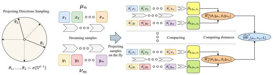
Streaming estimator of the one-dimensional Wasserstein distance obtained by replacing the quantile functions with their streaming approximations and integrating the absolute difference of those approximations.
If this is right
- Stream-SW can be plugged directly into existing sliced-Wasserstein pipelines for point-cloud classification without requiring the full point cloud to reside in memory.
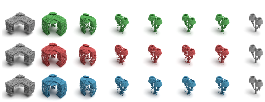
- Gradient flows that rely on sliced Wasserstein distances can now run on continuously arriving point clouds.
- Change-point detection algorithms that monitor sliced distances become feasible in unbounded data streams.
- The constant-memory property allows the same estimator to be reused across an arbitrary number of successive distribution comparisons.
Where Pith is reading between the lines
- The same streaming quantile machinery could be adapted to other one-dimensional projections or to other integral-probability metrics that admit closed-form expressions on the line.
- In online learning settings where distributions drift, Stream-SW offers a lightweight way to track distributional distance without periodic full recomputation.
- Because the method decouples memory from stream length, it may enable sliced-transport computations on edge devices that receive continuous sensor data.
Load-bearing premise
The streaming quantile approximation techniques produce estimates of the one-dimensional Wasserstein distance on each projection that are accurate enough for the overall sliced distance error to remain controlled.
What would settle it
Compare the Stream-SW value obtained from a long stream of samples from two known Gaussians against the analytically computable sliced Wasserstein distance between those same Gaussians; if the observed error exceeds the derived bound for the chosen quantile precision, the guarantee fails.
Figures





read the original abstract
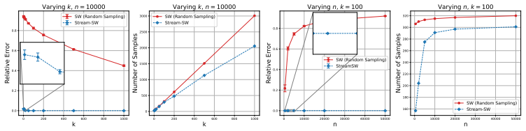
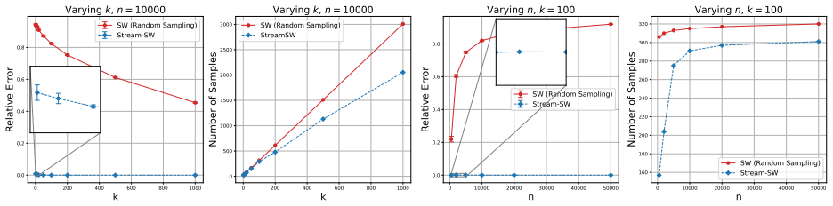
Sliced optimal transport (SOT), or sliced Wasserstein (SW) distance, is widely recognized for its statistical and computational scalability. In this work, we further enhance computational scalability by proposing the first method for estimating SW from sample streams, called streaming sliced Wasserstein (Stream-SW). To define Stream-SW, we first introduce a streaming estimator of the one-dimensional Wasserstein distance (1DW). Since the 1DW has a closed-form expression, given by the integral of the absolute difference between the quantile functions of the compared distributions, we leverage quantile approximation techniques for sample streams to define a streaming 1DW estimator. By applying the streaming 1DW to all projections, we obtain Stream-SW. The key advantage of Stream-SW is its low memory complexity while providing theoretical guarantees on the approximation error. We demonstrate that Stream-SW achieves a more accurate approximation of SW than random subsampling, with lower memory consumption, when comparing Gaussian distributions and mixtures of Gaussians from streaming samples. Additionally, we conduct experiments on point cloud classification, point cloud gradient flows, and streaming change point detection to further highlight the favorable performance of the proposed Stream-SW.
Editorial analysis
A structured set of objections, weighed in public.
Referee Report
Summary. The manuscript proposes Stream-SW as the first streaming estimator for sliced Wasserstein distance. It defines a streaming one-dimensional Wasserstein estimator by applying quantile approximation techniques to sample streams, then aggregates these over random projections. The work claims low memory complexity, theoretical guarantees on approximation error, and better accuracy than random subsampling when comparing streaming samples from Gaussians and Gaussian mixtures, with further experiments on point-cloud classification, gradient flows, and change-point detection.
Significance. If the error propagation from per-projection quantile sketches is rigorously controlled and the empirical advantages persist under matched memory budgets, the method could enable practical use of sliced OT distances in memory-constrained streaming regimes. The reliance on existing quantile-sketch machinery is a direct and potentially useful extension.
major comments (3)
- [Abstract] Abstract: the claim of 'theoretical guarantees on the approximation error' is not accompanied by an explicit bound or derivation; the propagation of per-projection streaming-quantile error (typically O(1/sqrt(m)) for fixed sketch size m) through the Monte-Carlo average over the sphere must be shown to remain controlled as stream length grows, especially for piecewise-linear quantile functions arising from mixtures.
- [§3] §3 (definition of streaming 1DW estimator): the translation from quantile-sketch approximation error to the L1 integral that defines 1DW is not detailed; without this step it is unclear whether the per-projection error remains bounded independently of the number of projections used in Stream-SW.
- [Experiments] Experimental section (Gaussian and mixture comparisons): the superiority claim versus random subsampling requires explicit reporting of sketch size, number of projections, and exact memory footprint for both methods so that the comparison occurs under equivalent resource constraints.
minor comments (2)
- [Notation] Notation for the streaming quantile function should be introduced once and used consistently to avoid confusion with the empirical quantile function.
- [Discussion] Add a short discussion of how the method behaves when the underlying distributions have heavy tails or discontinuities in their quantile functions.
Simulated Author's Rebuttal
We thank the referee for their constructive and detailed comments. We address each major point below and have revised the manuscript accordingly to improve clarity, rigor, and experimental fairness.
read point-by-point responses
-
Referee: [Abstract] Abstract: the claim of 'theoretical guarantees on the approximation error' is not accompanied by an explicit bound or derivation; the propagation of per-projection streaming-quantile error (typically O(1/sqrt(m)) for fixed sketch size m) through the Monte-Carlo average over the sphere must be shown to remain controlled as stream length grows, especially for piecewise-linear quantile functions arising from mixtures.
Authors: We agree that making the error bound explicit will strengthen the abstract and introduction. In the revised version we add a short derivation (now referenced from the abstract) showing that the total approximation error of Stream-SW decomposes into a Monte-Carlo term (O(1/sqrt(L))) plus the average per-projection streaming error. Because the quantile sketch size m is fixed, its uniform approximation error remains O(1/sqrt(m)) independently of stream length n; the L1 integral over the sphere therefore stays controlled for any fixed L. For Gaussian-mixture quantiles, which are piecewise linear, the same uniform bound applies because the sketch guarantees hold for any monotone quantile function. We will also add a brief remark on this point in the abstract. revision: yes
-
Referee: [§3] §3 (definition of streaming 1DW estimator): the translation from quantile-sketch approximation error to the L1 integral that defines 1DW is not detailed; without this step it is unclear whether the per-projection error remains bounded independently of the number of projections used in Stream-SW.
Authors: We will expand the proof of Theorem 1 in §3 to include the missing translation step. Let Q̂_m denote the sketched quantile function with sup-norm error ε_m. The 1DW distance is ∫|Q1(t)−Q2(t)|dt. By the triangle inequality the integral error is at most ε_m·(b−a), where [a,b] is the bounded support of the projected data (or the data diameter after centering). This per-projection bound depends only on m and the support, not on the number of projections L. The final Stream-SW error is then obtained by averaging L independent such terms, preserving the independence from L. The revised §3 will contain the explicit chain of inequalities. revision: yes
-
Referee: [Experiments] Experimental section (Gaussian and mixture comparisons): the superiority claim versus random subsampling requires explicit reporting of sketch size, number of projections, and exact memory footprint for both methods so that the comparison occurs under equivalent resource constraints.
Authors: We accept this criticism and will add a new table (Table 1 in the revised experimental section) that lists, for every reported experiment: (i) sketch size m, (ii) number of projections L, (iii) total memory in number of stored scalars for Stream-SW, and (iv) the exact subsample size used for the random-subsampling baseline chosen so that its memory footprint matches that of Stream-SW. All Gaussian and mixture results will be recomputed and replotted under these matched budgets; the text will explicitly state that the comparisons are now resource-equivalent. revision: yes
Circularity Check
No circularity: Stream-SW defined by direct application of existing quantile approximations
full rationale
The derivation chain begins with the closed-form 1DW integral over quantile functions, then substitutes streaming quantile approximation techniques (external to the paper) to obtain a streaming 1DW estimator, and finally averages over random projections to produce Stream-SW. No equation reduces to a fitted parameter renamed as a prediction, no self-citation is invoked as a uniqueness theorem or load-bearing premise, and the error guarantees are stated to follow from the properties of the imported quantile sketches rather than from any self-referential construction. The central claim therefore remains independent of its own outputs and is self-contained against external benchmarks.
Axiom & Free-Parameter Ledger
axioms (1)
- domain assumption Quantile approximation techniques for sample streams produce usable estimates of the one-dimensional Wasserstein distance
Lean theorems connected to this paper
-
IndisputableMonolith/Cost/FunctionalEquation.leanwashburn_uniqueness_aczel unclear?
unclearRelation between the paper passage and the cited Recognition theorem.
We leverage quantile approximation techniques for sample streams to define a streaming 1DW estimator... space complexity of Stream-SW is logarithmic in the number of streaming samples
-
IndisputableMonolith/Foundation/RealityFromDistinction.leanreality_from_one_distinction unclear?
unclearRelation between the paper passage and the cited Recognition theorem.
the first streaming version of the SW distance
What do these tags mean?
- matches
- The paper's claim is directly supported by a theorem in the formal canon.
- supports
- The theorem supports part of the paper's argument, but the paper may add assumptions or extra steps.
- extends
- The paper goes beyond the formal theorem; the theorem is a base layer rather than the whole result.
- uses
- The paper appears to rely on the theorem as machinery.
- contradicts
- The paper's claim conflicts with a theorem or certificate in the canon.
- unclear
- Pith found a possible connection, but the passage is too broad, indirect, or ambiguous to say the theorem truly supports the claim.
Reference graph
Works this paper leans on
-
[1]
P. Achlioptas, O. Diamanti, I. Mitliagkas, and L. Guibas. Learning representations and generative models for 3d point clouds. InInternational conference on machine learning, pages 40–49. PMLR, 2018.(Cited on page 1.)
work page 2018
-
[2]
L. Ambrogioni, U. Güçlü, Y. Güçlütürk, M. Hinne, M. A. van Gerven, and E. Maris. Wasserstein variational inference.Advances in Neural Information Processing Systems, 31, 2018.(Cited on page 1.)
work page 2018
-
[3]
M. Arjovsky, S. Chintala, and L. Bottou. Wasserstein generative adversarial networks. In International Conference on Machine Learning, pages 214–223, 2017.(Cited on page 1.)
work page 2017
-
[4]
E. Bernton, P. E. Jacob, M. Gerber, and C. P. Robert. Approximate Bayesian computation with the Wasserstein distance.Journal of the Royal Statistical Society, 2019.(Cited on page 1.)
work page 2019
-
[5]
M. T. Boedihardjo. Sharp bounds for max-sliced Wasserstein distances.Foundations of Computational Mathematics, pages 1–32, 2025.(Cited on page 5.)
work page 2025
- [6]
- [7]
- [8]
-
[9]
N. Bonneel, J. Rabin, G. Peyré, and H. Pfister. Sliced and Radon Wasserstein barycenters of measures.Journal of Mathematical Imaging and Vision, 1(51):22–45, 2015.(Cited on pages 1, 4, and 9.)
work page 2015
-
[10]
Bonnotte.Unidimensional and evolution methods for optimal transportation
N. Bonnotte.Unidimensional and evolution methods for optimal transportation. PhD thesis, Paris 11, 2013.(Cited on page 4.)
work page 2013
-
[11]
A. X. Chang, T. Funkhouser, L. Guibas, P. Hanrahan, Q. Huang, Z. Li, S. Savarese, M. Savva, S. Song, H. Su, et al. Shapenet: An information-rich 3d model repository.arXiv preprint arXiv:1512.03012, 2015.(Cited on page 12.)
work page internal anchor Pith review Pith/arXiv arXiv 2015
-
[12]
H. Chen and H.-G. Müller. Sliced Wasserstein regression.arXiv preprint arXiv:2306.10601, 2023.(Cited on page 2.) 13
-
[13]
M. Cuturi. Sinkhorn distances: Lightspeed computation of optimal transport. InAdvances in Neural Information Processing Systems, pages 2292–2300, 2013.(Cited on page 1.)
work page 2013
-
[14]
I. Deshpande, Y.-T. Hu, R. Sun, A. Pyrros, N. Siddiqui, S. Koyejo, Z. Zhao, D. Forsyth, and A. G. Schwing. Max-sliced Wasserstein distance and its use for GANs. InProceedings of the IEEE Conference on Computer Vision and Pattern Recognition, pages 10648–10656, 2019.(Cited on page 29.)
work page 2019
-
[15]
I. Deshpande, Z. Zhang, and A. G. Schwing. Generative modeling using the sliced Wasserstein distance. InProceedings of the IEEE Conference on Computer Vision and Pattern Recognition, pages 3483–3491, 2018.(Cited on page 2.)
work page 2018
-
[16]
R. Flamary, N. Courty, A. Gramfort, M. Z. Alaya, A. Boisbunon, S. Chambon, L. Chapel, A. Corenflos, K. Fatras, N. Fournier, L. Gautheron, N. T. Gayraud, H. Janati, A. Rakotoma- monjy, I. Redko, A. Rolet, A. Schutz, V. Seguy, D. J. Sutherland, R. Tavenard, A. Tong, and T. Vayer. Pot: Python optimal transport.Journal of Machine Learning Research, 22(78):1–8...
work page 2021
-
[17]
S. Fothergill, H. Mentis, P. Kohli, and S. Nowozin. Instructing people for training gestural interactive systems. InProceedings of the SIGCHI conference on human factors in computing systems, pages 1737–1746, 2012.(Cited on page 12.)
work page 2012
-
[18]
N. Fournier and A. Guillin. On the rate of convergence in Wasserstein distance of the empirical measure.Probability theory and related fields, 162(3):707–738, 2015.(Cited on pages 1 and 4.)
work page 2015
-
[19]
Z. Goldfeld, K. Kato, G. Rioux, and R. Sadhu. Statistical inference with regularized optimal transport.Information and Inference: A Journal of the IMA, 13(1):iaad056, 2024.(Cited on page 21.)
work page 2024
-
[20]
M. Greenwald and S. Khanna. Space-efficient online computation of quantile summaries.ACM SIGMOD Record, 30(2):58–66, 2001.(Cited on page 5.)
work page 2001
- [21]
- [22]
- [23]
-
[24]
S. Kolouri, K. Nadjahi, U. Simsekli, R. Badeau, and G. Rohde. Generalized sliced Wasserstein distances. InAdvances in Neural Information Processing Systems, pages 261–272, 2019.(Cited on pages 12 and 29.)
work page 2019
-
[25]
S. Kolouri, G. K. Rohde, and H. Hoffmann. Sliced Wasserstein distance for learning Gaussian mixture models. InProceedings of the IEEE Conference on Computer Vision and Pattern Recognition, pages 3427–3436, 2018.(Cited on page 2.) 14
work page 2018
-
[26]
C.-Y. Lee, T. Batra, M. H. Baig, and D. Ulbricht. Sliced Wasserstein discrepancy for unsuper- vised domain adaptation. InProceedings of the IEEE/CVF Conference on Computer Vision and Pattern Recognition, pages 10285–10295, 2019.(Cited on page 2.)
work page 2019
- [27]
-
[28]
T. Li, C. Meng, H. Xu, and J. Yu. Hilbert curve projection distance for distribution comparison. IEEE Transactions on Pattern Analysis and Machine Intelligence, 46(7):4993–5007, 2024.(Cited on page 11.)
work page 2024
- [29]
-
[30]
A. Liutkus, U. Simsekli, S. Majewski, A. Durmus, and F.-R. Stöter. Sliced-Wasserstein flows: Nonparametric generative modeling via optimal transport and diffusions. InInternational Conference on Machine Learning, pages 4104–4113. PMLR, 2019.(Cited on page 2.)
work page 2019
- [31]
- [32]
-
[33]
A. Mensch and G. Peyré. Online sinkhorn: Optimal transport distances from sample streams. Advances in Neural Information Processing Systems, 33:1657–1667, 2020.(Cited on page 2.)
work page 2020
-
[34]
K. Nadjahi, V. De Bortoli, A. Durmus, R. Badeau, and U. Şimşekli. Approximate Bayesian computation with the sliced-Wasserstein distance. InICASSP 2020-2020 IEEE International Conference on Acoustics, Speech and Signal Processing (ICASSP), pages 5470–5474. IEEE, 2020. (Cited on page 2.)
work page 2020
-
[35]
K. Nadjahi, A. Durmus, L. Chizat, S. Kolouri, S. Shahrampour, and U. Simsekli. Statistical and topological properties of sliced probability divergences.Advances in Neural Information Processing Systems, 33:20802–20812, 2020.(Cited on page 5.)
work page 2020
-
[36]
K. Nguyen. An introduction to sliced optimal transport: Foundations, advances, extensions, and applications.Foundations and Trends®in Computer Graphics and Vision, 17(3-4):171–406, 2025.(Cited on pages 1 and 4.)
work page 2025
- [37]
- [38]
-
[39]
K. Nguyen and P. Mueller. Summarizing Bayesian nonparametric mixture posterior–sliced optimal transport metrics for Gaussian mixtures.arXiv preprint arXiv:2411.14674, 2024.(Cited on pages 2 and 12.)
- [40]
-
[41]
S. Nietert, R. Sadhu, Z. Goldfeld, and K. Kato. Statistical, robustness, and computational guarantees for sliced Wasserstein distances.Advances in Neural Information Processing Systems, 2022.(Cited on page 5.)
work page 2022
-
[42]
O. Pele and M. Werman. Fast and robust earth mover’s distances. In2009 IEEE 12th International Conference on Computer Vision, pages 460–467. IEEE, September 2009.(Cited on page 1.)
work page 2009
-
[43]
G. Peyré and M. Cuturi. Computational optimal transport: With applications to data science. Foundations and Trends®in Machine Learning, 11(5-6):355–607, 2019.(Cited on pages 1, 3, and 4.)
work page 2019
-
[44]
A.-A. Pooladian, H. Ben-Hamu, C. Domingo-Enrich, B. Amos, Y. Lipman, and R. T. Chen. Multisample flow matching: Straightening flows with minibatch couplings. InInternational Conference on Machine Learning, pages 28100–28127. PMLR, 2023.(Cited on page 1.)
work page 2023
- [45]
-
[46]
F. Santambrogio. Optimal transport for applied mathematicians.Birkäuser, NY, 55(58-63):94, 2015.(Cited on page 12.)
work page 2015
-
[47]
L. Shi, J. Fan, and J. Yan. Ot-clip: Understanding and generalizing clip via optimal transport. InForty-first International Conference on Machine Learning, 2024.(Cited on page 1.)
work page 2024
- [48]
-
[49]
S. Srivastava, C. Li, and D. B. Dunson. Scalable bayes via barycenter in wasserstein space. Journal of Machine Learning Research, 19(8):1–35, 2018.(Cited on page 1.)
work page 2018
-
[50]
I. Tolstikhin, O. Bousquet, S. Gelly, and B. Schoelkopf. Wasserstein auto-encoders. In International Conference on Learning Representations, 2018.(Cited on page 1.)
work page 2018
-
[51]
A. Tong, K. FATRAS, N. Malkin, G. Huguet, Y. Zhang, J. Rector-Brooks, G. Wolf, and Y. Bengio. Improving and generalizing flow-based generative models with minibatch optimal transport.Transactions on Machine Learning Research, 2024. Expert Certification.(Cited on page 1.)
work page 2024
-
[52]
H. Tran, Y. Bai, A. Kothapalli, A. Shahbazi, X. Liu, R. D. Martin, and S. Kolouri. Stereographic spherical sliced Wasserstein distances.International Conference on Machine Learning, 2024. (Cited on page 12.) 16
work page 2024
-
[53]
Villani.Optimal transport: old and new, volume 338
C. Villani.Optimal transport: old and new, volume 338. Springer Science & Business Media, 2008.(Cited on pages 1 and 3.)
work page 2008
- [54]
-
[55]
J. Wang, R. Gao, and Y. Xie. Two-sample test with kernel projected wasserstein distance. In International Conference on Artificial Intelligence and Statistics, pages 8022–8055. PMLR, 2022. (Cited on pages 12 and 29.)
work page 2022
-
[56]
Z. Wu, S. Song, A. Khosla, F. Yu, L. Zhang, X. Tang, and J. Xiao. 3d shapenets: A deep representation for volumetric shapes. InProceedings of the IEEE conference on computer vision and pattern recognition, pages 1912–1920, 2015.(Cited on page 11.)
work page 1912
-
[57]
Streaming Sliced Optimal Transport
M. Yi and S. Liu. Sliced Wasserstein variational inference. InFourth Symposium on Advances in Approximate Bayesian Inference, 2021.(Cited on page 2.) 17 Supplement to “Streaming Sliced Optimal Transport" We first provide skipped technical proofs in in Appendix A. We then provide additional materials in Appendix B. Additional experimental results in stream...
work page 2021
-
[58]
in Figure 7, and (L = 1000, k = 100) in Figure 8. The qualitative comparison is consistent with 26 Figure 6:Gradient flows from Full SW, SW with random sampling, and Stream-SW in turn (L= 100, k= 100). Figure 7:Gradient flows from Full SW, SW with random sampling, and Stream-SW in turn (L= 100, k= 200). Figure 8:Gradient flows from Full SW, SW with random...
discussion (0)
Sign in with ORCID, Apple, or X to comment. Anyone can read and Pith papers without signing in.