Recognition: unknown
FLUID: Flow-based Unified Inference for Dynamics
Pith reviewed 2026-05-10 17:17 UTC · model grok-4.3
The pith
FLUID encodes variable-length observations into a fixed summary that conditions coupled forward and backward flows for unified filtering and smoothing.
A machine-rendered reading of the paper's core claim, the machinery that carries it, and where it could break.
Core claim
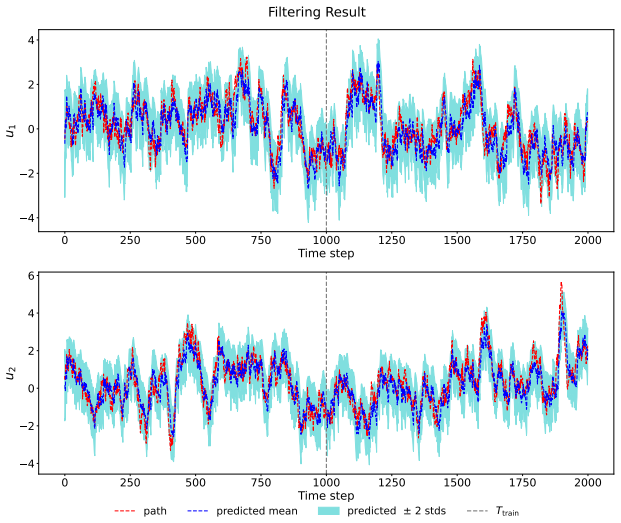
FLUID encodes each observation history into a fixed-dimensional summary statistic via a recurrent encoder. Conditioned on this statistic, a forward flow approximates the filtering distribution while a backward flow approximates the backward transition kernel. The smoothing distribution over an entire trajectory is recovered by combining the terminal filtering distribution with the learned backward flow through the standard backward recursion. By learning the underlying temporal evolution structure, FLUID also supports extrapolation beyond the training horizon.
What carries the argument
The fixed-dimensional recurrent summary statistic that is shared to condition both the forward filtering flow and the backward transition flow.
If this is right
- Accurate approximations of both filtering distributions and smoothing paths for high-dimensional nonlinear systems.
- Improved trajectory-level smoothing through implicit regularization induced by coupling the two flows via the shared summary.
- Extrapolation to time steps beyond the training horizon by learning the temporal evolution structure.
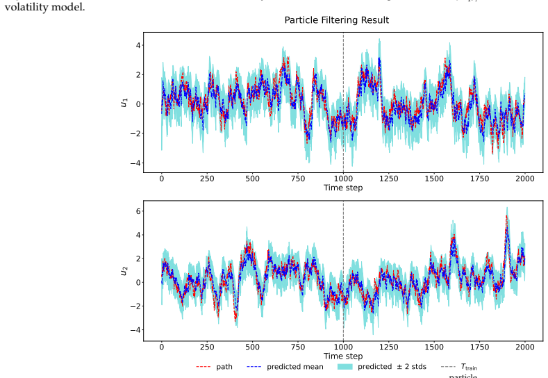
- An alternative flow-based particle filtering procedure with ESS-based diagnostics when explicit model factors are available.
Where Pith is reading between the lines
- The amortized nature of the shared summary could support repeated inference on new sequences at lower cost than retraining separate filters and smoothers.
- If the recurrent summary preserves the essential dynamics, the same trained flows might be reused on related systems that differ only in sequence length or noise level.
- Incremental updating of the recurrent summary as new observations arrive would allow the method to be applied in online settings without re-encoding the full history.
Load-bearing premise
A fixed-dimensional recurrent summary of the observation history is sufficient to condition accurate approximations of the filtering distribution and backward transition kernel for arbitrary-length sequences in high-dimensional nonlinear systems.
What would settle it
A test on a nonlinear system with long-range temporal dependencies where approximation error in the recovered smoothing paths increases sharply once sequence length exceeds the lengths used to train the recurrent encoder.
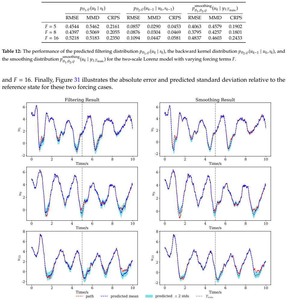
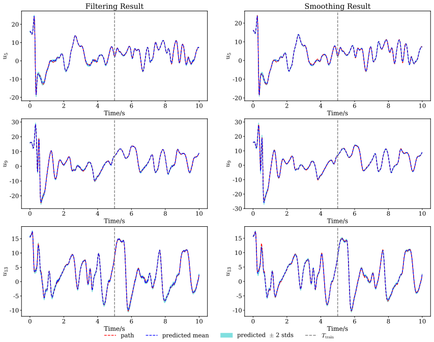
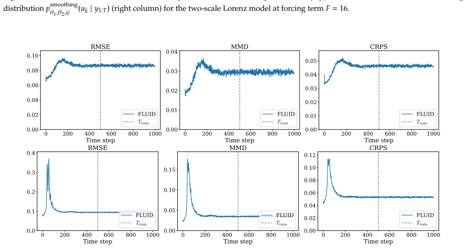
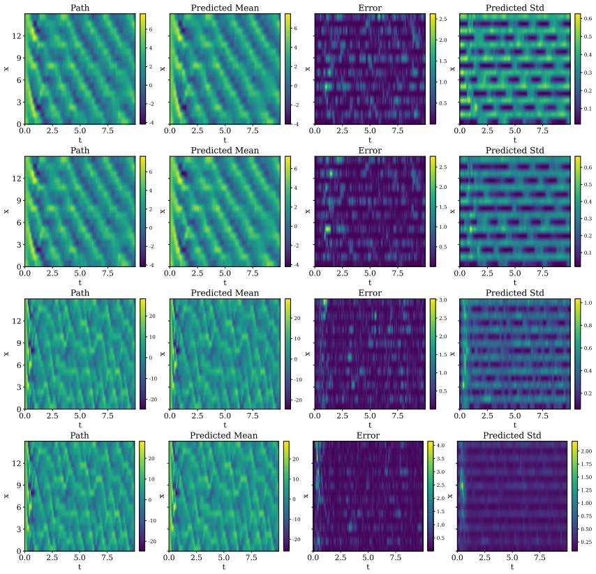
Figures


read the original abstract
Bayesian filtering and smoothing for high-dimensional nonlinear dynamical systems are fundamental yet challenging problems in many areas of science and engineering. In this work, we propose FLUID, a flow-based unified amortized inference framework for filtering and smoothing dynamics. The core idea is to encode each observation history into a fixed-dimensional summary statistic and use this shared representation to learn both a forward flow for the filtering distribution and a backward flow for the backward transition kernel. Specifically, a recurrent encoder maps each observation history to a fixed-dimensional summary statistic whose dimension does not depend on the length of the time series. Conditioned on this shared summary statistic, the forward flow approximates the filtering distribution, while the backward flow approximates the backward transition kernel. The smoothing distribution over an entire trajectory is then recovered by combining the terminal filtering distribution with the learned backward flow through the standard backward recursion. By learning the underlying temporal evolution structure, FLUID also supports extrapolation beyond the training horizon. Moreover, by coupling the two flows through shared summary statistics, FLUID induces an implicit regularization across latent state trajectories and improves trajectory-level smoothing. In addition, we develop a flow-based particle filtering variant that provides an alternative filtering procedure and enables ESS-based diagnostics when explicit model factors are available. Numerical experiments demonstrate that FLUID provides accurate approximations of both filtering distributions and smoothing paths.
Editorial analysis
A structured set of objections, weighed in public.
Referee Report
Summary. The manuscript introduces FLUID, a flow-based unified amortized inference framework for Bayesian filtering and smoothing in high-dimensional nonlinear dynamical systems. A recurrent encoder maps observation histories to fixed-dimensional summary statistics independent of sequence length; conditioned on this shared summary, a forward flow approximates the filtering distribution while a backward flow approximates the backward transition kernel. Smoothing distributions are recovered via standard backward recursion, with additional claims of support for extrapolation beyond training horizons, implicit regularization across trajectories from the shared summary, and a flow-based particle filtering variant. Numerical experiments are stated to demonstrate accurate approximations of both filtering distributions and smoothing paths.
Significance. If the central claims hold, FLUID would offer a scalable amortized approach to joint filtering and smoothing that couples the two tasks through shared representations, potentially improving trajectory-level accuracy via implicit regularization while enabling extrapolation. The flow-based formulation provides flexible density modeling without explicit model factors in the base procedure, and the particle-filtering extension adds diagnostic capabilities when factors are available. These features could advance inference in complex state-space models common in science and engineering.
major comments (2)
- [§3] §3 (Method): The central claim that a fixed-dimensional recurrent summary serves as a sufficient statistic for both the filtering distribution (forward flow) and the backward transition kernel (backward flow) for arbitrary-length sequences in high-dimensional nonlinear systems is load-bearing for the smoothing recursion and the implicit-regularization argument, yet no theoretical justification, information-loss bounds, or ablation on summary dimension versus sequence length is provided to support sufficiency.
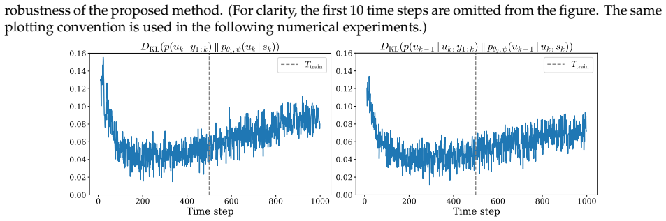
- [§5] §5 (Numerical Experiments): The assertion that experiments demonstrate accurate approximations lacks specification of baselines (e.g., standard particle filters, other amortized methods), quantitative metrics (KL, ESS, trajectory error), data regimes (state dimension, sequence lengths, nonlinearity), or controls for hyperparameter selection, which directly undermines evaluation of the claimed improvements in filtering and smoothing.
minor comments (1)
- [Abstract and §3] The abstract and method sections use 'shared summary statistic' without an explicit equation defining its dimension or the recurrent encoder architecture (e.g., LSTM vs. GRU hidden size), which would improve reproducibility.
Simulated Author's Rebuttal
Thank you for the constructive review and for recognizing the potential of FLUID as a scalable amortized approach to joint filtering and smoothing. We address each major comment below and commit to revisions that strengthen the manuscript without altering its core contributions.
read point-by-point responses
-
Referee: [§3] §3 (Method): The central claim that a fixed-dimensional recurrent summary serves as a sufficient statistic for both the filtering distribution (forward flow) and the backward transition kernel (backward flow) for arbitrary-length sequences in high-dimensional nonlinear systems is load-bearing for the smoothing recursion and the implicit-regularization argument, yet no theoretical justification, information-loss bounds, or ablation on summary dimension versus sequence length is provided to support sufficiency.
Authors: We agree that a formal theoretical guarantee of sufficiency would provide stronger support. The recurrent encoder is motivated by the universal approximation capabilities of RNNs for sequence compression, which have been effective in related dynamical modeling tasks. In the revised manuscript we will expand the discussion in §3 to clarify the modeling assumptions and add an ablation study that varies summary dimension against sequence length, reporting effects on filtering and smoothing accuracy. This supplies the requested empirical assessment while preserving the practical emphasis of the work. revision: yes
-
Referee: [§5] §5 (Numerical Experiments): The assertion that experiments demonstrate accurate approximations lacks specification of baselines (e.g., standard particle filters, other amortized methods), quantitative metrics (KL, ESS, trajectory error), data regimes (state dimension, sequence lengths, nonlinearity), or controls for hyperparameter selection, which directly undermines evaluation of the claimed improvements in filtering and smoothing.
Authors: We appreciate the referee highlighting the need for clearer experimental reporting. The original manuscript contains comparisons and metrics, but these details were insufficiently explicit. We will revise §5 to list all baselines (including particle filters and other amortized methods), report quantitative results using KL divergence, effective sample size, and trajectory errors, specify data regimes (state dimensions, sequence lengths, nonlinearity levels), and describe hyperparameter selection with controls. These updates will make the evaluation transparent and reproducible. revision: yes
Circularity Check
No circularity: standard flows, recurrent summary, and backward recursion remain independent of fitted outputs
full rationale
The derivation encodes observation histories via a recurrent network into a fixed-dimensional summary, then trains separate normalizing flows for the filtering distribution and backward kernel conditioned on that summary. Smoothing is recovered by applying the textbook backward recursion to the terminal filter and the learned backward kernel. None of these steps re-uses a fitted quantity as its own prediction, invokes a self-citation for a uniqueness theorem, or smuggles an ansatz through prior work. The shared-summary coupling is an architectural choice whose regularization effect is asserted but not derived by re-labeling inputs; numerical validation is external to the algebraic chain. The procedure is therefore self-contained against external benchmarks and receives score 0.
Axiom & Free-Parameter Ledger
free parameters (1)
- dimension of summary statistic
axioms (2)
- domain assumption Normalizing flows can accurately approximate the filtering distribution and backward transition kernel when conditioned on the summary statistic
- domain assumption The recurrent encoder compresses arbitrary-length histories into a fixed vector without critical information loss for the inference task
invented entities (1)
-
shared summary statistic produced by recurrent encoder
no independent evidence
Forward citations
Cited by 2 Pith papers
-
One Operator for Many Densities: Amortized Approximation of Conditioning by Neural Operators
A single neural operator can approximate the map from arbitrary joint densities to their conditionals, backed by new continuity results and illustrated on Gaussian mixtures.
-
One Operator for Many Densities: Amortized Approximation of Conditioning by Neural Operators
A single neural operator can approximate the map from joint densities to conditional densities to arbitrary accuracy, with a proof based on continuity of the conditioning operator and a demonstration on Gaussian mixtures.
Reference graph
Works this paper leans on
-
[1]
Särkkä, L
S. Särkkä, L. Svensson, Bayesian filtering and smoothing, volume 17, Cambridge university press, 2023
2023
-
[2]
K. Law, A. Stuart, K. Zygalakis, Data assimilation, Cham, Switzerland: Springer 214 (2015) 7
2015
-
[3]
M. Asch, M. Bocquet, M. Nodet, Data assimilation: methods, algorithms, and applications, SIAM, 2016
2016
-
[5]
J. Ko, D. Fox, GP-BayesFilters: Bayesian filtering using Gaussian process prediction and observation models, Autonomous Robots 27 (2009) 75–90
2009
-
[6]
J. V . Candy, Bayesian signal processing: classical, modern, and particle filtering methods, John Wiley & Sons, 2016
2016
-
[7]
H. F. Lopes, R. S. Tsay, Particle filters and Bayesian inference in financial econometrics, Journal of Forecasting 30 (2011) 168–209
2011
-
[8]
Zhang, M
X. Zhang, M. L. King, Box-Cox stochastic volatility models with heavy-tails and correlated errors, Journal of Empirical Finance 15 (2008) 549–566
2008
-
[9]
Chopin, Central Limit Theorem for sequential Monte Carlo methods and its application to Bayesian inference, Annals of Statistics 32 (2004) 2385–2411
N. Chopin, Central Limit Theorem for sequential Monte Carlo methods and its application to Bayesian inference, Annals of Statistics 32 (2004) 2385–2411
2004
-
[10]
Bengtsson, P
T. Bengtsson, P . Bickel, B. Li, Curse-of-dimensionality revisited: Collapse of the particle filter in very large scale systems, in: Probability and statistics: Essays in honor of David A. Freedman, volume 2, Institute of Mathematical Statistics, 2008, pp. 316–335
2008
-
[11]
Rebeschini, R
P . Rebeschini, R. van Handel, Can local particle filters beat the curse of dimensionality?, The Annals of Applied Probability (2015)
2015
-
[12]
R. E. Kalman, A new approach to linear filtering and prediction problems (1960)
1960
-
[13]
G. A. Einicke, L. B. White, Robust extended Kalman filtering, IEEE transactions on signal processing 47 (2002) 2596–2599
2002
-
[14]
Evensen, The ensemble Kalman filter: Theoretical formulation and practical implementation, Ocean dynamics 53 (2003) 343–367
G. Evensen, The ensemble Kalman filter: Theoretical formulation and practical implementation, Ocean dynamics 53 (2003) 343–367
2003
-
[15]
Calvello, S
E. Calvello, S. Reich, A. M. Stuart, Ensemble Kalman methods: A mean-field perspective, Acta Numerica 34 (2025) 123–291
2025
-
[16]
Doucet, N
A. Doucet, N. De Freitas, N. J. Gordon, et al., Sequential Monte Carlo methods in practice, volume 1, Springer, 2001
2001
-
[17]
Beskos, A
A. Beskos, A. Jasra, E. A. Muzaffer, A. M. Stuart, Sequential Monte Carlo methods for Bayesian elliptic inverse problems, Statistics and Computing 25 (2015) 727–737
2015
-
[18]
P . M. Djuric, J. H. Kotecha, J. Zhang, Y. Huang, T. Ghirmai, M. F. Bugallo, J. Miguez, Particle filtering, IEEE signal processing magazine 20 (2003) 19–38
2003
-
[19]
N. J. Gordon, D. J. Salmond, A. F. Smith, Novel approach to nonlinear/non-Gaussian Bayesian state estimation, in: IEE proceedings F (radar and signal processing), volume 140, IET, pp. 107–113
-
[20]
M. K. Pitt, N. Shephard, Filtering via simulation: Auxiliary particle filters, Journal of the American statistical association 94 (1999) 590–599
1999
-
[21]
Carpenter, P
J. Carpenter, P . Clifford, P . Fearnhead, Improved particle filter for nonlinear problems, IEE Proceedings- Radar, Sonar and Navigation 146 (1999) 2–7. 41
1999
-
[22]
Kitagawa, Monte Carlo filter and smoother for non-Gaussian nonlinear state space models, Journal of computational and graphical statistics 5 (1996) 1–25
G. Kitagawa, Monte Carlo filter and smoother for non-Gaussian nonlinear state space models, Journal of computational and graphical statistics 5 (1996) 1–25
1996
-
[23]
W. R. Gilks, C. Berzuini, Following a moving target—Monte Carlo inference for dynamic Bayesian models, Journal of the Royal Statistical Society: Series B (Statistical Methodology) 63 (2001) 127–146
2001
-
[24]
Snyder, T
C. Snyder, T. Bengtsson, P . Bickel, J. Anderson, Obstacles to high-dimensional particle filtering, Monthly Weather Review 136 (2008) 4629–4640
2008
-
[25]
Reich, C
S. Reich, C. Cotter, Probabilistic forecasting and Bayesian data assimilation, Cambridge University Press, 2015
2015
-
[26]
Del Moral, A
P . Del Moral, A. Doucet, A. Jasra, On adaptive resampling strategies for sequential Monte Carlo methods (2012)
2012
-
[27]
Cheng, C
S. Cheng, C. Quilodrán-Casas, S. Ouala, A. Farchi, C. Liu, P . Tandeo, R. Fablet, D. Lucor, B. Iooss, J. Brajard, et al., Machine learning with data assimilation and uncertainty quantification for dynamical systems: a review, IEEE/CAA Journal of Automatica Sinica 10 (2023) 1361–1387
2023
- [28]
-
[29]
X.-H. Zhou, Z.-R. Liu, H. Xiao, BI-EqNO: Generalized approximate Bayesian inference with an equiv- ariant neural operator framework, arXiv preprint arXiv:2410.16420 (2024)
-
[30]
Bocquet, A
M. Bocquet, A. Farchi, T. S. Finn, C. Durand, S. Cheng, Y. Chen, I. Pasmans, A. Carrassi, Accurate deep learning-based filtering for chaotic dynamics by identifying instabilities without an ensemble, Chaos: An Interdisciplinary Journal of Nonlinear Science 34 (2024)
2024
- [31]
-
[32]
Revach, N
G. Revach, N. Shlezinger, X. Ni, A. L. Escoriza, R. J. Van Sloun, Y. C. Eldar, KalmanNet: Neural network aided Kalman filtering for partially known dynamics, IEEE Transactions on Signal Processing 70 (2022) 1532–1547
2022
-
[33]
F. Bao, Z. Zhang, G. Zhang, A score-based filter for nonlinear data assimilation, Journal of Computa- tional Physics 514 (2024) 113207
2024
-
[34]
F. Bao, Z. Zhang, G. Zhang, An ensemble score filter for tracking high-dimensional nonlinear dynamical systems, Computer Methods in Applied Mechanics and Engineering 432 (2024) 117447
2024
-
[35]
P . T. Huynh, G. Zhang, F. Bao, et al., Joint State-Parameter Estimation for the Reduced Fracture Model via the United Filter, Journal of Computational Physics (2025) 114159
2025
- [36]
-
[37]
X. T. Tong, Y. Wang, L. Yan, Latent Autoencoder Ensemble Kalman Filter for Data assimilation, arXiv preprint arXiv:2603.06752 (2026)
work page internal anchor Pith review Pith/arXiv arXiv 2026
-
[38]
Taghvaei, P
A. Taghvaei, P . G. Mehta, An optimal transport formulation of the ensemble Kalman filter, IEEE Transactions on Automatic Control 66 (2020) 3052–3067
2020
-
[39]
Spantini, R
A. Spantini, R. Baptista, Y. Marzouk, Coupling techniques for nonlinear ensemble filtering, SIAM Review 64 (2022) 921–953
2022
-
[40]
M. Ramgraber, D. Sharp, M. L. Provost, Y. Marzouk, A friendly introduction to triangular transport, arXiv preprint arXiv:2503.21673 (2025). 42
-
[41]
Y. Zhao, T. Cui, Tensor-train methods for sequential state and parameter learning in state-space models, Journal of Machine Learning Research 25 (2024) 1–51
2024
-
[42]
Kobyzev, S
I. Kobyzev, S. J. Prince, M. A. Brubaker, Normalizing flows: An introduction and review of current methods, IEEE transactions on pattern analysis and machine intelligence 43 (2020) 3964–3979
2020
-
[43]
Papamakarios, E
G. Papamakarios, E. Nalisnick, D. J. Rezende, S. Mohamed, B. Lakshminarayanan, Normalizing flows for probabilistic modeling and inference, Journal of Machine Learning Research 22 (2021) 1–64
2021
-
[44]
Zammit-Mangion, M
A. Zammit-Mangion, M. Sainsbury-Dale, R. Huser, Neural methods for amortized inference, Annual Review of Statistics and Its Application 12 (2025) 311–335
2025
-
[45]
M. Deistler, J. Boelts, P . Steinbach, G. Moss, T. Moreau, M. Gloeckler, P . L. Rodrigues, J. Linhart, J. K. Lappalainen, B. K. Miller, et al., Simulation-based inference: A practical guide, arXiv preprint arXiv:2508.12939 (2025)
- [46]
-
[47]
X. Feng, L. Zeng, T. Zhou, Solving Time Dependent Fokker-Planck Equations via Temporal Normalizing Flow, Communications in Computational Physics 32 (2022) 401–423
2022
-
[48]
J. He, Q. Liao, X. Wan, Adaptive deep density approximation for stochastic dynamical systems, Journal of Scientific Computing 102 (2025) 57
2025
-
[49]
Doucet, S
A. Doucet, S. Godsill, C. Andrieu, On sequential Monte Carlo sampling methods for Bayesian filtering, Statistics and computing 10 (2000) 197–208
2000
-
[50]
D. S. Wilks, Effects of stochastic parametrizations in the Lorenz’96 system, Quarterly Journal of the Royal Meteorological Society: A journal of the atmospheric sciences, applied meteorology and physical oceanography 131 (2005) 389–407. 43
2005
discussion (0)
Sign in with ORCID, Apple, or X to comment. Anyone can read and Pith papers without signing in.