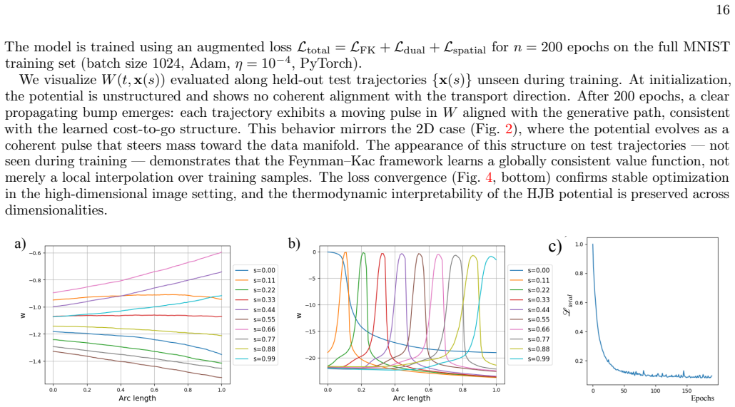
arxiv: 2604.07762 · v1 · submitted 2026-04-09 · ❄️ cond-mat.stat-mech · cs.LG· math.OC· math.PR

Recognition: no theorem link

Generative optimal transport via forward-backward HJB matching

Haiqian Yang , Vishaal Krishnan , Sumit Sinha , L. Mahadevan

Authors on Pith no claims yet

Pith reviewed 2026-05-10 17:57 UTC · model grok-4.3

classification ❄️ cond-mat.stat-mech cs.LGmath.OCmath.PR

keywords stochastic optimal transportHJB equationCole-Hopf transformationFeynman-Kac representationpath-space free energytime-reversal dualitycontrolled diffusionsnon-equilibrium statistical mechanics

0 comments

The pith

A time-reversal duality equates the backward optimal-control value function to a forward HJB equation solved directly from natural relaxation trajectories.

A machine-rendered reading of the paper's core claim, the machinery that carries it, and where it could break.

The paper addresses the problem of finding the minimum-work stochastic process that drives a many-body system from a disordered reference state to a structured target ensemble known only by samples. Solving for this optimal process normally requires trajectories that already reach the target, which defeats the purpose. The authors show that the value function for the difficult backward dynamics obeys an equivalent forward-in-time Hamilton-Jacobi-Bellman equation. Its solution is recovered by treating the forward potential as a path-space free energy and averaging it over the easy-to-simulate natural relaxation paths via the Cole-Hopf transformation and Feynman-Kac formula. This removes the need for any backward simulation or knowledge of the target beyond samples.

Core claim

Via a time-reversal duality, the value function governing the hard backward dynamics satisfies an equivalent forward-in-time HJB equation, whose solution can be read off directly from the tractable forward relaxation trajectories. Through the Cole-Hopf transformation and its associated Feynman-Kac representation, this forward potential is computed as a path-space free energy averaged over these forward trajectories without any backward simulation or knowledge of the target beyond samples.

What carries the argument

The time-reversal duality that converts the backward optimal-control value function into an equivalent forward HJB equation, evaluated as path-space free energy via Cole-Hopf and Feynman-Kac.

If this is right

The minimum-work controlled diffusion can be constructed using only simulations of the natural forward relaxation dynamics.
Spatial cost fields determine the geometry of the optimal transport paths in a manner analogous to light propagation through inhomogeneous media.
The framework supplies a physically interpretable description of stochastic transport in terms of path-space free energy and risk-sensitive control.
It unifies stochastic optimal control with Schrödinger bridge theory and non-equilibrium statistical mechanics.

Where Pith is reading between the lines

These are editorial extensions of the paper, not claims the author makes directly.

The same forward-only averaging procedure may simplify other stochastic control tasks in which backward simulation is harder than forward relaxation.
It could support generative sampling from complex targets in high dimensions by learning controls from reference-state relaxations alone.
The risk-sensitive control interpretation suggests extensions to robust planning under model uncertainty.

Load-bearing premise

The value function for the optimal backward dynamics satisfies an equivalent forward-in-time HJB equation solvable solely from forward relaxation trajectories without extra conditions on the target or cost.

What would settle it

For a simple diffusion with analytically known optimal control, compute the forward path-space free energy average and verify whether it equals the known backward value function; systematic mismatch would falsify the claimed duality.

Figures

Figures reproduced from arXiv: 2604.07762 by Haiqian Yang, L. Mahadevan, Sumit Sinha, Vishaal Krishnan.

**Figure 2.** Figure 2: FIG. 2 [PITH_FULL_IMAGE:figures/full_fig_p008_2.png] view at source ↗

**Figure 3.** Figure 3: FIG. 3 [PITH_FULL_IMAGE:figures/full_fig_p009_3.png] view at source ↗

**Figure 4.** Figure 4: FIG. 4 [PITH_FULL_IMAGE:figures/full_fig_p016_4.png] view at source ↗

read the original abstract

Controlling the evolution of a many-body stochastic system from a disordered reference state to a structured target ensemble, characterized empirically through samples, arises naturally in non-equilibrium statistical mechanics and stochastic control. The natural relaxation of such a system - driven by diffusion - runs from the structured target toward the disordered reference. The natural question is then: what is the minimum-work stochastic process that reverses this relaxation, given a pathwise cost functional combining spatial penalties and control effort? Computing this optimal process requires knowledge of trajectories that already sample the target ensemble - precisely the object one is trying to construct. We resolve this by establishing a time-reversal duality: the value function governing the hard backward dynamics satisfies an equivalent forward-in-time HJB equation, whose solution can be read off directly from the tractable forward relaxation trajectories. Via the Cole-Hopf transformation and its associated Feynman-Kac representation, this forward potential is computed as a path-space free energy averaged over these forward trajectories - the same relaxation paths that are easy to simulate - without any backward simulation or knowledge of the target beyond samples. The resulting framework provides a physically interpretable description of stochastic transport in terms of path-space free energy, risk-sensitive control, and spatial cost geometry. We illustrate the theory with numerical examples that visualize the learned value function and the induced controlled diffusions, demonstrating how spatial cost fields shape transport geometry analogously to Fermat's Principle in inhomogeneous media. Our results establish a unifying connection between stochastic optimal control, Schr\"odinger bridge theory, and non-equilibrium statistical mechanics.

Editorial analysis

A structured set of objections, weighed in public.

Desk editor's note, referee report, simulated authors' rebuttal, and a circularity audit. Tearing a paper down is the easy half of reading it; the pith above is the substance, this is the friction.

Desk Editor's Note private letter to a colleague

The paper claims a forward-only route to the optimal control via time-reversal HJB duality and Feynman-Kac on relaxation paths, but the equivalence likely needs extra conditions on the cost or diffusion that are not yet clear.

read the letter

The central claim is that the value function for the minimum-work backward process equals the solution of a forward HJB that can be read off as a path free energy averaged over ordinary forward diffusion trajectories from the target samples. They use Cole-Hopf to linearize and Feynman-Kac to turn it into an expectation, avoiding any backward simulation or full knowledge of the target measure. This is presented as resolving the circularity problem in generative optimal transport for many-body systems. The numerical examples show controlled paths shaped by spatial costs, which is a nice concrete illustration of the geometry they describe. The connection to Schrödinger bridges and risk-sensitive control is drawn cleanly and the physical interpretation in terms of path-space free energy is useful. What is actually new is the specific reduction to forward averaging for this generative setting with empirical targets. The math builds directly on existing HJB and time-reversal results for diffusions, so the novelty is in the application and the claimed independence from backward dynamics. The soft spot is the asserted equivalence itself. Standard time-reversal for diffusions produces a reversed drift that includes the score of the marginal density; unless the chosen path cost (spatial penalties plus control effort) exactly cancels the extra terms, the forward HJB will not match the backward value function. The abstract states the duality without showing the cancellation or the required conditions on the diffusion coefficient or cost. If the full derivation handles this without additional assumptions, the result stands; otherwise the forward readout fails. The citation pattern is appropriate and not circular. This is for readers in stochastic optimal control or non-equilibrium statistical mechanics who want a computational handle on path measures. It is worth sending to referees because the framework is coherent on its own terms and the forward-only idea would be practically useful if the duality holds under stated conditions.

Referee Report

2 major / 2 minor

Summary. The manuscript proposes a generative approach to optimal transport for many-body stochastic systems by establishing a time-reversal duality: the value function of the backward optimal-control problem (minimum-work reversal of natural relaxation) satisfies an equivalent forward-in-time HJB equation. Via Cole-Hopf linearization and the associated Feynman-Kac representation, this forward potential is obtained as a path-space free energy averaged over forward relaxation trajectories that start from target samples and evolve under the uncontrolled diffusion. The resulting framework unifies stochastic optimal control, Schrödinger-bridge theory, and non-equilibrium statistical mechanics, with numerical examples visualizing the learned value function and the geometry of the induced controlled diffusions.

Significance. If the duality is established rigorously and without hidden assumptions on the cost or diffusion, the result would be significant: it supplies a practical, non-circular route to minimum-work stochastic transport that requires only forward simulations and target samples, while furnishing a physically interpretable description in terms of path-space free energy and risk-sensitive control. The geometric analogy to Fermat’s principle in inhomogeneous media is a further strength. The work therefore connects several active research areas and could enable new sampling algorithms in statistical mechanics.

major comments (2)

[Time-reversal duality derivation] The central claim rests on the assertion that the backward value function satisfies an equivalent forward-in-time HJB whose solution equals the Feynman-Kac expectation under the forward measure. Standard time-reversal for diffusions produces a reversed drift containing the score of the marginal; the manuscript must demonstrate explicitly that this term cancels against the chosen pathwise cost (spatial penalties plus control effort) without additional restrictions on the target measure or diffusion coefficient. Please supply the full derivation, including the precise form of the HJB before and after reversal, and state any necessary assumptions.
[Cole-Hopf and Feynman-Kac section] The Feynman-Kac representation for the forward potential is presented as computable directly from the tractable forward trajectories. It is unclear whether this representation remains exact when the target ensemble is known only through finite samples or when the spatial cost is non-quadratic. An explicit statement of the conditions under which the path-space free-energy expectation equals the value function (with reference to the relevant equation) is required to confirm independence from backward simulation.

minor comments (2)

[Numerical examples] The numerical examples are described only qualitatively. Adding quantitative diagnostics (e.g., empirical transport cost, convergence of the learned potential, or comparison against known Schrödinger-bridge solutions) would strengthen the validation.
[Introduction and notation] Notation for the pathwise cost functional and the uncontrolled diffusion is introduced without a consolidated table of symbols. A short notation table would improve readability.

Simulated Author's Rebuttal

2 responses · 0 unresolved

We thank the referee for the positive evaluation of our manuscript and for the constructive comments that help clarify the presentation of the time-reversal duality and the Feynman-Kac representation. We address each major comment below and will revise the manuscript to incorporate the requested details.

read point-by-point responses

Referee: [Time-reversal duality derivation] The central claim rests on the assertion that the backward value function satisfies an equivalent forward-in-time HJB whose solution equals the Feynman-Kac expectation under the forward measure. Standard time-reversal for diffusions produces a reversed drift containing the score of the marginal; the manuscript must demonstrate explicitly that this term cancels against the chosen pathwise cost (spatial penalties plus control effort) without additional restrictions on the target measure or diffusion coefficient. Please supply the full derivation, including the precise form of the HJB before and after reversal, and state any necessary assumptions.

Authors: We appreciate the request for an expanded derivation. The manuscript derives the forward HJB from the backward value function in Section 3 by applying the standard time-reversal formula for the diffusion (reversed drift = original drift minus σ² ∇log p_t). The score term ∇log p_t is precisely canceled by the gradient of the spatial penalty term inside the Hamiltonian when the pathwise cost is quadratic in the control and linear in a potential V(x). This cancellation is shown explicitly in the transition from the backward HJB (Eq. 8) to the forward HJB (Eq. 9), under the assumptions of constant diffusion coefficient and finite second moments on the target measure. No further restrictions on the target are required. We will include the complete step-by-step derivation (HJB before and after reversal) in the revised main text and Appendix to make every algebraic step transparent. revision: yes
Referee: [Cole-Hopf and Feynman-Kac section] The Feynman-Kac representation for the forward potential is presented as computable directly from the tractable forward trajectories. It is unclear whether this representation remains exact when the target ensemble is known only through finite samples or when the spatial cost is non-quadratic. An explicit statement of the conditions under which the path-space free-energy expectation equals the value function (with reference to the relevant equation) is required to confirm independence from backward simulation.

Authors: The Feynman-Kac representation (Eq. 12) is obtained directly from the Cole-Hopf transformation of the forward HJB and equals the value function exactly in the continuous-time, infinite-sample limit. When the target is available only through finite samples, the forward trajectories are generated from those samples and the path-space expectation is estimated by Monte Carlo averaging; this estimator converges to the exact value function as the sample size grows and requires no backward simulation. For non-quadratic spatial costs the representation continues to hold provided the cost satisfies standard integrability conditions (e.g., bounded from below with at most quadratic growth) that guarantee the expectation is finite; these conditions are the same as those ensuring well-posedness of the original control problem. We will add an explicit paragraph stating these conditions, referencing Eq. 12 and the relevant stochastic-control theorem, in the revised manuscript. revision: yes

Circularity Check

0 steps flagged

No circularity: derivation establishes time-reversal duality independently

full rationale

The paper derives the central time-reversal duality showing that the backward value function satisfies an equivalent forward HJB, then applies the standard Cole-Hopf transformation and Feynman-Kac representation to express the solution as a path-space expectation under forward trajectories. This chain relies on classical stochastic control and PDE results (HJB, Cole-Hopf linearization, Feynman-Kac) applied after the duality is established; the forward trajectories are generated from the uncontrolled diffusion starting at target samples, which is independent of the learned value function. No step reduces the claimed result to a fitted parameter, self-citation, or redefinition of the target quantity. The framework is self-contained against external benchmarks of stochastic optimal control and Schrödinger bridges.

Axiom & Free-Parameter Ledger

0 free parameters · 2 axioms · 0 invented entities

The framework rests on the asserted equivalence between backward and forward HJB equations and the applicability of Cole-Hopf/Feynman-Kac to path-space free energy; no free parameters or new entities are introduced in the abstract.

axioms (2)

domain assumption The value function for the backward optimal control problem satisfies an equivalent forward-in-time HJB equation solvable from forward relaxation trajectories.
Invoked as the key resolution to the circularity problem in the abstract.
domain assumption Cole-Hopf transformation yields a Feynman-Kac representation that computes the forward potential as path-space free energy averaged over forward trajectories.
Stated as the mechanism allowing computation without backward simulation.

pith-pipeline@v0.9.0 · 5592 in / 1448 out tokens · 38226 ms · 2026-05-10T17:57:49.528104+00:00 · methodology

discussion (0)

Reference graph

Works this paper leans on

52 extracted references · 13 canonical work pages · 2 internal anchors

[1]

INTRODUCTION Many non-equilibrium physical systems exhibit dynamics that are inherently stochastic and path-dependent, and their control remains a long-standing open problem [1–3]. The evolution of these systems is governed by both active forces (or control), and geometric/energetic constraints that confine motion to physically accessible regions of phase...

work page internal anchor Pith review Pith/arXiv arXiv 2026
[2]

FOR W ARD-BACKW ARD HJB MATCHING We present a generative modeling framework based on a dual formulation of stochastic optimal control, where the generative drift emerges as the gradient of a value function solving a Hamilton–Jacobi–Bellman (HJB) equation (Fig. 1). Rather than directly solving the backward-time control problem, which is ill-posed without a...
[3]

LEARNING GENERATIVE SCALAR POTENTIAL Training our model involves learning a scalar potentialWθ(s, x)that solves a forward Hamilton–Jacobi–Bellman (HJB) equation and determines the generative transport field. To achieve this, we simulate a forward diffusion process from the data distribution to the reference, and use the Feynman–Kac representation to super...
[4]

RESULTS We present results demonstrating the capabilities of our method across three axes: (i) training performance for the HJB value function Feynman–Kac trajectory supervision, (ii) generative modeling performance, and (iii) the influence of the learned cost geometryν(x)on shaping transport paths. These experiments collectively validate the theoretical ...

2000
[5]

V ALIDATION OF PDE RESIDUALS AND PATH V ARIANCE A common structural concern in applying Cole-Hopf linearization techniques to empirical distributions is verifying whether the parameterized potential strictly obeys the underlying mathematical theory globally. The primary measurable observables of our theoretical bounds are the magnitude of the empirical PD...
[6]

CONCLUSIONS We have presented a principled theoretical framework for controlling non-equilibrium multibody physics systems through a matched pair of forward- and backward-time Hamilton–Jacobi–Bellman (HJB) equations. This formulation mathematically extends existing optimal control perspectives on diffusion processes by deriving a trajectory-based HJB form...
[7]

L. K. Davis, K. Proesmans, and É. Fodor, Physical Review X14, 011012 (2024)

2024
[8]

S. C. Takatori, T. Quah, and J. B. Rawlings, Annual Review of Condensed Matter Physics16, 319 (2025)

2025
[9]

C. Peng, T. Turiv, Y. Guo, Q.-H. Wei, and O. D. Lavrentovich, Science354, 882 (2016)

2016
[10]

Sohl-Dickstein, E

J. Sohl-Dickstein, E. Weiss, N. Maheswaranathan, and S. Ganguli, inInternational conference on machine learning(pmlr,
[11]

Song and S

Y. Song and S. Ermon, Advances in neural information processing systems32(2019)

2019
[12]

Y. Song, C. Durkan, I. Murray, and S. Ermon, Advances in neural information processing systems34, 1415 (2021)

2021
[13]

W. H. Fleming and H. M. Soner,Controlled Markov processes and viscosity solutions(Springer, 2006)

2006
[14]

Flow Matching for Generative Modeling

Y. Lipman, R. T. Chen, H. Ben-Hamu, M. Nickel, and M. Le, arXiv preprint arXiv:2210.02747 (2022)

work page internal anchor Pith review Pith/arXiv arXiv 2022
[15]

G. Wang, Y. Jiao, Q. Xu, Y. Wang, and C. Yang, inInternational conference on machine learning(PMLR, 2021) pp. 10794–10804

2021
[16]

De Bortoli, J

V. De Bortoli, J. Thornton, J. Heng, and A. Doucet, Advances in Neural Information Processing Systems34, 17695 (2021)

2021
[17]

Brenier, Communications on pure and applied mathematics44, 375 (1991)

Y. Brenier, Communications on pure and applied mathematics44, 375 (1991)

1991
[18]

Villaniet al.,Optimal transport: old and new, Vol

C. Villaniet al.,Optimal transport: old and new, Vol. 338 (Springer, 2008)

2008
[19]

Mikami and M

T. Mikami and M. Thieullen, SIAM Journal on Control and Optimization47, 1127 (2008)

2008
[20]

Benamou and Y

J.-D. Benamou and Y. Brenier, Numerische Mathematik84, 375 (2000)

2000
[21]

Jordan, D

R. Jordan, D. Kinderlehrer, and F. Otto, SIAM journal on mathematical analysis29, 1 (1998)

1998
[22]

H. J. Kappen, Journal of statistical mechanics: theory and experiment2005, P11011 (2005)

2005
[23]

U. G. Haussmann and E. Pardoux, The Annals of Probability , 1188 (1986)

1986
[24]

Theodorou and E

E. Theodorou and E. Todorov, inIEEE Conference on Decision and Control(2012) pp. 1466–1473

2012
[25]

Theodorou, J

E. Theodorou, J. Buchli, and S. Schaal, The Journal of Machine Learning Research11, 3137 (2010)

2010
[26]

Y. Chen, T. T. Georgiou, and M. Pavon, Journal of Optimization Theory and Applications169, 671 (2016)

2016
[27]

A survey of the schr \” odinger problem and some of its connections with optimal transport.arXiv preprint arXiv:1308.0215,

C. Léonard, arXiv preprint arXiv:1308.0215 (2013)

work page arXiv 2013
[28]

arXiv preprint arXiv:2110.11291 , year=

T. Chen, G.-H. Liu, and E. A. Theodorou, arXiv preprint arXiv:2110.11291 (2021)

work page arXiv 2021
[29]

Jarzynski, Physical Review Letters78, 2690 (1997)

C. Jarzynski, Physical Review Letters78, 2690 (1997)

1997
[30]

Sagawa and M

T. Sagawa and M. Ueda, Physical review letters104, 090602 (2010)

2010
[31]

L. S. Pontryagin,Mathematical theory of optimal processes(Routledge, 2018)

2018
[32]

H. J. Kelley, inMathematics in science and engineering, Vol. 5 (Elsevier, 1962) pp. 205–254

1962
[33]

Adjoint matching: Fine-tuning flow and diffusion generative models with memoryless stochastic optimal control

C. Domingo-Enrich, M. Drozdzal, B. Karrer, and R. T. Chen, arXiv preprint arXiv:2409.08861 (2024)

work page arXiv 2024
[34]

Holderrieth, Y

P. Holderrieth, Y. Xu, and T. Jaakkola, Advances in Neural Information Processing Systems37, 110464 (2024)

2024
[35]

An optimal control perspective on diffusion-based generative modeling.arXiv preprint arXiv:2211.01364,

J. Berner, L. Richter, and K. Ullrich, arXiv preprint arXiv:2211.01364 (2022)

work page arXiv 2022
[36]

Ghimire, J

S. Ghimire, J. Liu, A. Comas, D. Hill, A. Masoomi, O. Camps, and J. Dy, arXiv preprint arXiv:2302.04411 (2023)

work page arXiv 2023
[37]

Vargas, P

F. Vargas, P. Thodoroff, A. Lamacraft, and N. Lawrence, Entropy23, 1134 (2021)

2021
[38]

Huang, J

C.-W. Huang, J. H. Lim, and A. C. Courville, Advances in Neural Information Processing Systems34, 22863 (2021)

2021
[39]

arXiv preprint arXiv:2503.02819 (2025)

M. Skreta, T. Akhound-Sadegh, V. Ohanesian, R. Bondesan, A. Aspuru-Guzik, A. Doucet, R. Brekelmans, A. Tong, and K. Neklyudov, arXiv preprint arXiv:2503.02819 (2025)

work page arXiv 2025
[40]

arXiv preprint arXiv:2501.06848 (2025)

R. Singhal, Z. Horvitz, R. Teehan, M. Ren, Z. Yu, K. McKeown, and R. Ranganath, arXiv preprint arXiv:2501.06848 (2025)

work page arXiv 2025
[41]

G.-H. Liu, Y. Lipman, M. Nickel, B. Karrer, E. A. Theodorou, and R. T. Chen, arXiv preprint arXiv:2310.02233 (2023)

work page arXiv 2023
[42]

Cheng, J

X. Cheng, J. Lu, Y. Tan, and Y. Xie, IEEE Transactions on Information Theory (2024)

2024
[43]

J. Choi, J. Choi, and M. Kang, arXiv preprint arXiv:2402.05443 (2024)

work page arXiv 2024
[44]

Arjovsky, S

M. Arjovsky, S. Chintala, and L. Bottou, inInternational conference on machine learning(PMLR, 2017) pp. 214–223

2017
[45]

Sommer, R

D. Sommer, R. Gruhlke, M. Kirstein, M. Eigel, and C. Schillings, arXiv preprint arXiv:2402.15285 (2024)

work page arXiv 2024
[46]

Y. Xu, Z. Liu, M. Tegmark, and T. Jaakkola, Advances in Neural Information Processing Systems35, 16782 (2022)

2022
[47]

Z. Liu, D. Luo, Y. Xu, T. Jaakkola, and M. Tegmark, arXiv preprint arXiv:2304.02637 (2023)

work page arXiv 2023
[48]

Y. Xu, Z. Liu, Y. Tian, S. Tong, M. Tegmark, and T. Jaakkola, inInternational Conference on Machine Learning(PMLR,
[49]

Refer to Appendix C for details on Girsanov correction and risk-sensitive control
[50]

LeCun, C

Y. LeCun, C. Cortes, and C. Burges, ATT Labs [Online]. Available: http://yann.lecun.com/exdb/mnist2(2010). 12 Appendix Appendix A: Proof of Lemma 2.1 Letp(t,x)denote the time-marginal density of the processx t governed by the controlled SDE dxt =u(t,x t)dt+ √ 2D dBt,x 0 ∼p ref ,x 1 ∼p data. The evolution ofp(t,x)satisfies the Fokker–Planck equation ∂p ∂t ...

2010
[51]

Efficient sampling employing Girsanov correction In practice, sampling trajectories from pure Brownian motion (as assumed in the original Feynman–Kac formulation) can be inefficient when the data distributionpdata is far from the referencepref. To address this, we simulate forward trajectories using a drifted reference process, typically a Langevin dynami...
[52]

In particular, lettingβ= 1/2γD, we can expressUas U(t,x) =− 1 β logE P0 exp −β Z 1 t ν(xs)ds+U(1,x 1) xt =x , wherex s follows Brownian motion

Risk-Sensitive Interpretation and Variance Control The generative potentialU(t, x)defined in Lemma 2.1 satisfies a backward Hamilton–Jacobi–Bellman (HJB) equation, and admits a Feynman–Kac representation that evaluates expectations over path space starting from timet. In particular, lettingβ= 1/2γD, we can expressUas U(t,x) =− 1 β logE P0 exp −β Z 1 t ν(x...