Recognition: unknown
Medial Axis Aware Learning of Signed Distance Functions
Pith reviewed 2026-05-10 13:10 UTC · model grok-4.3
The pith
A variational method computes highly accurate global signed distance functions from point clouds by modeling their medial axis.
A machine-rendered reading of the paper's core claim, the machinery that carries it, and where it could break.
Core claim
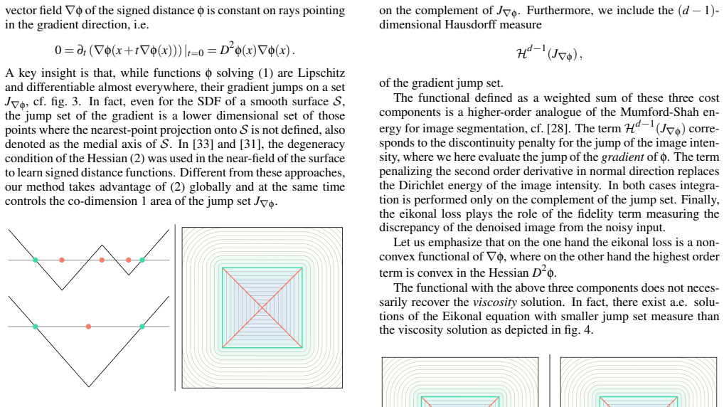
By taking the jump set of the gradient of the signed distance function, which is the medial axis, explicitly into account in a higher-order variational formulation that enforces linear growth along the gradient direction, and using a phase field approximation of Ambrosio-Tortorelli type to make the problem tractable, the method produces a global SDF that satisfies the eikonal equation and accurately represents the distance to the point cloud surface.
What carries the argument
The higher-order variational formulation enforcing linear growth along the gradient away from the medial axis discontinuity, approximated by a phase field function that implicitly describes the medial axis.
If this is right
- The SDF satisfies the eikonal equation as a hard constraint.
- Linear growth is enforced away from the medial axis, improving global accuracy.
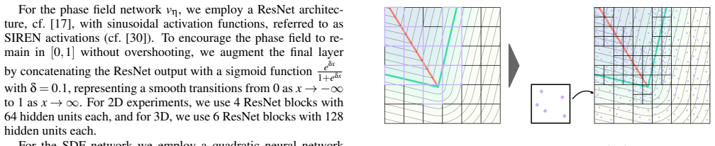
- Neural networks can jointly approximate the SDF and the phase field for unoriented point clouds.
- Quantitative comparisons demonstrate better performance than existing methods in both near-field and far-field regions.
Where Pith is reading between the lines
- Such medial axis awareness could enhance other distance-based computations in computer vision and geometry processing.
- Extending the method to time-dependent or deformable surfaces might yield more robust tracking.
- Applying similar higher-order terms to other variational problems involving discontinuities could improve solutions in related fields.
Load-bearing premise
The phase field approximation of the medial axis is accurate enough that the higher-order term can enforce linear growth without creating artifacts or breaking the eikonal constraint.
What would settle it
Compute the medial axis from a known closed surface, train the method on a point cloud sampled from it, and check if the learned function's gradient discontinuity set matches the true medial axis and if the growth is exactly linear.
Figures


read the original abstract
We propose a novel variational method to compute a highly accurate global signed distance function (SDF) to a given point cloud. To this end, the jump set of the gradient of the SDF, which coincides with the medial axis of the surface, is explicitly taken into account through a higher-order variational formulation that enforces linear growth along the gradient direction away from this discontinuity set. The eikonal equation and the zero-level set of the SDF are enforced as constraints. To make this variational problem computationally tractable, a phase field approximation of Ambrosio-Tortorelli type is employed. The associated phase field function implicitly describes the medial axis. The method is implemented for surfaces represented by unoriented point clouds using neural network approximations of both the SDF and the phase field. Experiments demonstrate the method's accuracy both in the near field and globally. Quantitative and qualitative comparisons with other approaches show the advantages of the proposed method.
Editorial analysis
A structured set of objections, weighed in public.
Referee Report
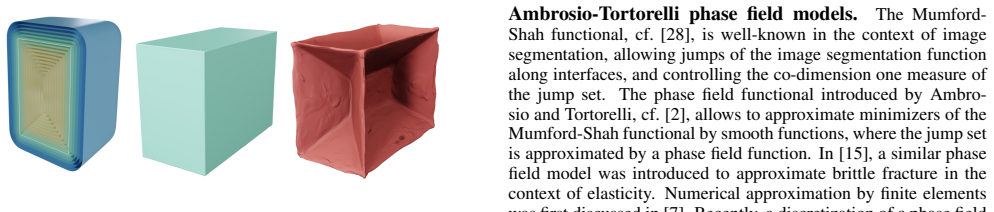
Summary. The paper proposes a novel variational method to compute a highly accurate global signed distance function (SDF) from an unoriented point cloud by explicitly incorporating the medial axis (the jump set of the SDF gradient) via a higher-order formulation that enforces linear growth along gradient directions away from this set. The eikonal equation and zero level-set are enforced as constraints, with an Ambrosio-Tortorelli phase-field approximation used to implicitly describe the medial axis; both the SDF and phase field are represented by neural networks, and experiments claim improved accuracy in near-field and global regimes relative to prior approaches.
Significance. If the central construction holds, the work would offer a meaningful advance in neural implicit geometry by making the medial axis an explicit part of the variational objective rather than an emergent property. This could yield more reliable global SDFs for downstream tasks such as collision detection, path planning, and surface reconstruction from sparse or noisy data. The combination of higher-order regularization with a phase-field relaxation and neural parameterization is technically interesting and, if supported by rigorous validation, would strengthen the literature on constrained implicit representations.
major comments (2)
- [variational formulation and phase-field approximation] The load-bearing assumption is that the jointly optimized Ambrosio-Tortorelli phase field φ recovers the (possibly non-unique) medial axis with sufficient fidelity that the higher-order linear-growth term can enforce u(x) ≈ u(y) + |x-y| along rays normal to the jump set while |∇u|=1 holds almost everywhere outside the diffuse interface. No derivation or consistency analysis of the coupled Euler-Lagrange equations is supplied to show that residual curvature or gradient jumps inside the ε-transition zone are prevented; this directly affects whether the eikonal constraint remains satisfied where the new penalty is active.
- [experiments and implementation] The experimental section reports qualitative and quantitative advantages but supplies neither the precise loss terms used to enforce the eikonal and zero-level-set constraints inside the neural optimization nor ablation studies that isolate the contribution of the higher-order medial-axis term. Without these, it is impossible to verify that observed improvements stem from the claimed mechanism rather than from network capacity or hyper-parameter tuning.
minor comments (2)
- [method] The notation distinguishing the phase-field variable φ from the SDF u should be introduced earlier and kept consistent when the Ambrosio-Tortorelli functional is first written.
- [figures] Figure captions would benefit from explicit statements of point-cloud density, sampling strategy, and the value of ε employed in each visualized result.
Simulated Author's Rebuttal
We thank the referee for the constructive feedback on our manuscript. The comments highlight important aspects of the variational formulation and experimental validation that we will address in the revision. We provide detailed responses below.
read point-by-point responses
-
Referee: [variational formulation and phase-field approximation] The load-bearing assumption is that the jointly optimized Ambrosio-Tortorelli phase field φ recovers the (possibly non-unique) medial axis with sufficient fidelity that the higher-order linear-growth term can enforce u(x) ≈ u(y) + |x-y| along rays normal to the jump set while |∇u|=1 holds almost everywhere outside the diffuse interface. No derivation or consistency analysis of the coupled Euler-Lagrange equations is supplied to show that residual curvature or gradient jumps inside the ε-transition zone are prevented; this directly affects whether the eikonal constraint remains satisfied where the new penalty is active.
Authors: We agree that a more detailed analysis of the variational problem would strengthen the manuscript. The Ambrosio-Tortorelli approximation is chosen because it is known to Γ-converge to the Mumford-Shah functional, which in this context approximates the jump set of the gradient. The higher-order term is added to enforce the linear growth property characteristic of the signed distance function away from the medial axis. To address the concern regarding the Euler-Lagrange equations and consistency in the transition zone, we will include in the revised manuscript a derivation of the stationarity conditions for the coupled system and a discussion of how the eikonal constraint is preserved outside the ε-interface, supported by theoretical references and numerical verification. revision: yes
-
Referee: [experiments and implementation] The experimental section reports qualitative and quantitative advantages but supplies neither the precise loss terms used to enforce the eikonal and zero-level-set constraints inside the neural optimization nor ablation studies that isolate the contribution of the higher-order medial-axis term. Without these, it is impossible to verify that observed improvements stem from the claimed mechanism rather than from network capacity or hyper-parameter tuning.
Authors: We acknowledge that providing the exact loss formulations and ablation studies is essential for reproducibility and to validate the contribution of each component. To fully address this comment, we will add a dedicated subsection detailing all loss terms with their weights used in the neural optimization, and include ablation experiments that compare the full model against variants without the higher-order medial axis term. These additions will be incorporated in the revised version. revision: yes
Circularity Check
No circularity: formulation rests on standard eikonal and Ambrosio-Tortorelli phase-field concepts
full rationale
The paper proposes a variational method enforcing the eikonal equation and linear growth away from the medial axis (identified with the jump set of ∇u) via a higher-order term, approximated by an Ambrosio-Tortorelli phase field. These are established external techniques; the abstract and described construction do not reduce any prediction or central quantity to a fit on the same data, a self-citation chain, or a definitional renaming. Neural-network approximations of u and φ are standard function approximators, not a source of circularity. No load-bearing step equates an output to its input by construction. The method is therefore self-contained against external benchmarks.
Axiom & Free-Parameter Ledger
axioms (2)
- domain assumption The jump set of the gradient of the SDF coincides with the medial axis of the surface
- domain assumption The eikonal equation and zero-level set condition can be enforced as constraints in the variational problem
Reference graph
Works this paper leans on
-
[1]
AMBROSIO, C
L. AMBROSIO, C. DELELLIS,ANDC. MANTEGAZZA, Line energies for gradient vector fields in the plane, Calcu- lus of Variations and Partial Differential Equations, 9 (1999), pp. 327–355
1999
-
[2]
AMBROSIO ANDV
L. AMBROSIO ANDV. M. TORTORELLI,On the approxi- mation of free discontinuity problems, Bollettino dell’Unione Matematica Italiana, Sezione B, 6 (1992), pp. 105–123
1992
-
[3]
AVILES ANDY
P. AVILES ANDY. GIGA,A mathematical problem related to the physical theory of liquid crystal configurations, Proc. Centre Math. Anal. Austral. Nat. Univ., 12 (1987), pp. 1–16
1987
-
[4]
,The distance function and defect energy, Proceedings of the Royal Society of Edinburgh: Section A Mathematics, 126 (1996), p. 923–938
1996
-
[5]
BEN-SHABAT, C
Y. BEN-SHABAT, C. H. KONEPUTUGODAGE,AND S. GOULD,Digs: Divergence guided shape implicit neural representation for unoriented point clouds, in Proceedings of the IEEE/CVF Conference on Computer Vision and Pattern Recognition, New Orleans, USA, 2022, pp. 19323–19332
2022
-
[6]
BERGER, J
M. BERGER, J. A. LEVINE, L. G. NONATO, G. TAUBIN, ANDC. T. SILVA,A benchmark for surface reconstruction, ACM Trans. Graph., 32 (2013)
2013
-
[7]
BOURDIN, G
B. BOURDIN, G. FRANCFORT,ANDJ.-J. MARIGO,Numer- ical experiments in revisited brittle fracture, Journal of the Mechanics and Physics of Solids, 48 (2000), pp. 797–826
2000
-
[8]
COIFFIER ANDL
G. COIFFIER ANDL. BÉTHUNE,1-Lipschitz neural distance fields, in Computer Graphics Forum, vol. 43, Wiley Online Library, 2024, p. e15128
2024
-
[9]
CRANE, C
K. CRANE, C. WEISCHEDEL,ANDM. WARDETZKY, Geodesics in heat: A new approach to computing distance based on heat flow, ACM Transactions on Graphics (TOG), 32 (2013), pp. 1–11
2013
-
[10]
,The heat method for distance computation, Commu- nications of the ACM, 60 (2017), pp. 90–99
2017
-
[11]
ESSAKINE, Y
A. ESSAKINE, Y. CHENG, C.-W. CHENG, L. ZHANG, Z. DENG, L. ZHU, C.-B. SCHÖNLIEB,ANDA. I. AVILES- RIVERO,Where do we stand with implicit neural representa- tions? a technical and performance survey, Transactions on Machine Learning Research, (2025). Survey Certification
2025
-
[12]
L. C. EVANS,Partial Differential Equations, American Mathematical Society, 1998
1998
-
[13]
F. FAN, J. XIONG,ANDG. WANG,Universal approximation with quadratic deep networks, Neural Networks, 124 (2020), pp. 383–392
2020
-
[14]
FENG ANDK
N. FENG ANDK. CRANE,A heat method for generalized signed distance, ACM Trans. Graph., 43 (2024)
2024
-
[15]
FRANCFORT ANDJ.-J
G. FRANCFORT ANDJ.-J. MARIGO,Revisiting brittle frac- ture as an energy minimization problem, Journal of the Me- chanics and Physics of Solids, 46 (1998), pp. 1319–1342
1998
-
[16]
J. C. HART,Sphere tracing: a geometric method for the an- tialiased ray tracing of implicit surfaces, The Visual Com- puter, 12 (1996), pp. 527–545
1996
-
[17]
K. HE, X. ZHANG, S. REN,ANDJ. SUN,Deep residual learning for image recognition, 2016 IEEE Conference on Computer Vision and Pattern Recognition (CVPR), (2015), pp. 770–778
2016
-
[18]
JIN ANDR
W. JIN ANDR. V. KOHN,Singular perturbation and the energy of folds, Journal of Nonlinear Science, 10 (2000), pp. 355–390
2000
-
[19]
D. P. KINGMA ANDJ. BA,Adam: A method for stochastic optimization, CoRR, abs/1412.6980 (2014)
work page internal anchor Pith review Pith/arXiv arXiv 2014
-
[20]
KLEINEBERG,Mesh-to-sdf: Calculate signed distance fields for arbitrary meshes, 2021
M. KLEINEBERG,Mesh-to-sdf: Calculate signed distance fields for arbitrary meshes, 2021
2021
-
[21]
C. D. LELLIS,An example in the gradient theory of phase transitions, ESAIM: Control, Optimisation and Calculus of Variations, 7 (2002), pp. 285–289
2002
-
[22]
LIPMAN,Phase transitions, distance functions, and im- plicit neural representations, in International Conference on Machine Learning, 2021
Y. LIPMAN,Phase transitions, distance functions, and im- plicit neural representations, in International Conference on Machine Learning, 2021
2021
-
[23]
P. LIU, Y. ZHANG, H. WANG, M. K. YIP, E. S. LIU,AND X. JIN,Real-time collision detection between general SDFs, Computer Aided Geometric Design, 111 (2024), p. 102305
2024
-
[24]
MANAV, R
M. MANAV, R. MOLINARO, S. MISHRA,ANDL. DE LORENZIS,Phase-field modeling of fracture with physics- informed deep learning, Computer Methods in Applied Me- chanics and Engineering, 429 (2024), p. 117104
2024
-
[25]
MARSCHNER, S
Z. MARSCHNER, S. SELLÁN, H.-T. D. LIU,ANDA. JA- COBSON,Constructive solid geometry on neural signed dis- tance fields, in SIGGRAPH Asia 2023 conference papers, Sydney, Australia, 2023, pp. 1–12
2023
-
[26]
MEHTA, M
I. MEHTA, M. CHANDRAKER,ANDR. RAMAMOORTHI,A level set theory for neural implicit evolution under explicit flows, in European Conference on Computer Vision, Tel Aviv, Israel, 2022, Springer, pp. 711–729
2022
-
[27]
MODICA ANDS
L. MODICA ANDS. MORTOLA,Un esempio diΓ- convergenza, Boll. Un. Mat. Ital. B (5), 14 (1977), pp. 285– 299
1977
-
[28]
MUMFORD ANDJ
D. MUMFORD ANDJ. SHAH,Optimal approximations by piecewise smooth functions and associated variational prob- lems, Comm. Pure Appl. Math., 42 (1989), pp. 577–685
1989
-
[29]
PASZKE, S
A. PASZKE, S. GROSS, F. MASSA, A. LERER, J. BRAD- BURY, G. CHANAN, T. KILLEEN, Z. LIN, N. GIMELSHEIN, L. ANTIGA, A. DESMAISON, A. KÖPF, E. YANG, Z. DE- VITO, M. RAISON, A. TEJANI, S. CHILAMKURTHY, B. STEINER, L. FANG, J. BAI,ANDS. CHINTALA,PyTorch: an imperative style, high-performance deep learning library, Curran Associates Inc., Red Hook, NY , USA, 2019
2019
-
[30]
SITZMANN, J
V. SITZMANN, J. N. P. MARTEL, A. W. BERGMAN, D. B. LINDELL,ANDG. WETZSTEIN,Implicit neural representa- tions with periodic activation functions, 2020
2020
-
[31]
R. WANG, Z. WANG, Y. ZHANG, S. CHEN, S. XIN, C. TU, ANDW. WANG,Aligning gradient and hessian for neural signed distance function, in Advances in Neural Informa- tion Processing Systems, A. Oh, T. Naumann, A. Globerson, K. Saenko, M. Hardt, and S. Levine, eds., vol. 36, Curran Associates, Inc., 2023, pp. 63515–63528
2023
-
[32]
Z. WANG, C. WANG, T. YOSHINO, S. TAO, Z. FU,ANDT.- M. LI,Hotspot: Signed distance function optimization with an asymptotically sufficient condition, in CVPR, 2025
2025
-
[33]
Z. WANG, Y. ZHANG, R. XU, F. ZHANG, P.-S. WANG, S. CHEN, S. XIN, W. WANG,ANDC. TU,Neural-singular- Hessian: Implicit neural representation of unoriented point clouds by enforcing singular Hessian, ACM Transactions on Graphics (TOG), 42 (2023), pp. 1–14. 10
2023
-
[34]
WEIDEMAIER, F
S. WEIDEMAIER, F. HARTWIG, J. SASSEN, S. CONTI, M. BEN-CHEN,ANDM. RUMPF,Sdfs from unoriented point clouds using neural variational heat distances, Computer Graphics Forum, n/a (2026), p. e70296
2026
-
[35]
H. YANG, Y. SUN, G. SUNDARAMOORTHI,ANDA. YEZZI, Steik: stabilizing the optimization of neural signed distance functions and finer shape representation, in Proceedings of the 37th International Conference on Neural Information Pro- cessing Systems, NIPS ’23, Red Hook, USA, 2023, Curran Associates Inc
2023
-
[36]
YEH, C.-H
I.-C. YEH, C.-H. LIN, O. SORKINE,ANDT.-Y. LEE, Template-based 3d model fitting using dual-domain relax- ation, IEEE Transactions on Visualization and Computer Graphics, 17 (2010), pp. 1178–1190
2010
-
[37]
Q. ZHOU ANDA. JACOBSON,Thingi10k: A dataset of 10,000 3d-printing models, Preprint arXiv:1605.04797, (2016). A Proof of theorem 3.1 For every(φ,v)∈H 2(Ω)×H 1(Ω), the total lossLε total[φ,v]is finite. Let(φ ε i ,v ε i )i∈N ⊂H 2(Ω)×H 1(Ω)be a minimizing sequence, i.e. inf (φ,v) Lε total[φ,v] =lim i→∞ Lε total[φε i ,v ε i ]≤C<∞. Using this boundedness and th...
discussion (0)
Sign in with ORCID, Apple, or X to comment. Anyone can read and Pith papers without signing in.