Recognition: unknown
A fully parallel densely connected probabilistic Ising machine with inertia for real-time applications
Pith reviewed 2026-05-10 06:47 UTC · model grok-4.3
The pith
Adding an inertia term to Ising spin dynamics enables fully parallel synchronous updates while improving success probability on dense problems.
A machine-rendered reading of the paper's core claim, the machinery that carries it, and where it could break.
Core claim
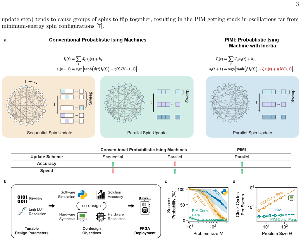
A modified Ising spin dynamics with an added inertia term permits fully parallel, synchronous updates in densely connected probabilistic Ising machines, enabling speed advantages that grow faster than linearly with the number of spins while maintaining or improving success probability on Max-Cut, Sherrington-Kirkpatrick, and MIMO detection instances.
What carries the argument
The inertia term added to the probabilistic bit (p-bit) update rule, which stabilizes the parallel synchronous dynamics so that they continue to optimize toward the target distribution.
If this is right
- Fully parallel updates produce a speed advantage that grows faster than linearly with the number of spins.
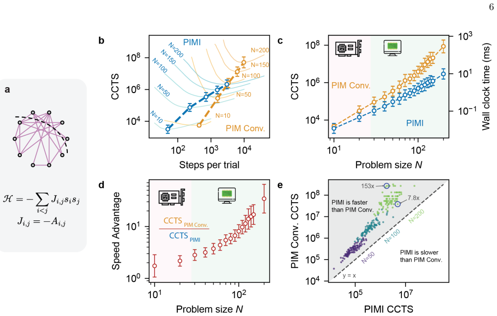
- Average speedup of approximately 35 times for 200-spin Max-Cut and SK-1 problems, with single-instance cases reaching 150 times.
- Co-design of the dynamics with hardware implementation meets solution quality and latency requirements for real-time 5G MIMO detection using practical silicon area.
Where Pith is reading between the lines
- Hardware designs could scale to larger spin counts without the sequential-update bottleneck limiting throughput.
- The inertia modification might extend to other probabilistic computing schemes that currently rely on asynchronous updates.
- Broader testing across graph densities and additional application domains would be needed to establish the limits of the observed performance gains.
Load-bearing premise
The inertia-modified parallel dynamics continue to sample from the correct Boltzmann distribution for arbitrary dense graphs.
What would settle it
A measurement on a new dense Max-Cut or SK instance showing that parallel inertia updates yield lower success probability than sequential updates on the same instance.
Figures


read the original abstract
Ising machines -- special-purpose hardware for heuristically solving Ising optimization problems -- based on probabilistic bits (p-bits) have been established as a promising alternative to heuristic optimization algorithms run on conventional computers. However, it has -- until now -- been thought that Ising spins that are connected in probabilistic Ising machines cannot be updated in parallel without ruining the machine's solving ability. This has been a major challenge for using probabilistic Ising machines as fast solvers for densely connected problems. Here, we circumvent this by introducing a modified Ising spin dynamics with an added inertia term, and verify in algorithm simulations, FPGA hardware emulation, and FPGA experiments that it enables fully parallel, synchronous updates while improving rather than degrading success probability. We evaluated on various types of abstract (Max-Cut and Sherrington-Kirkpatrick-model) and application-derived (MIMO, wireless detection) dense Ising benchmark instances. Performing fully parallel updates results in a speed advantage that grows faster than linearly with the number of spins, giving rise to large time-to-solution increases for practical problem sizes. For both Max-Cut and the SK-1 model at a problem size of 200, our approach achieved an average speedup of $\approx 35\times$, with the best single-instance speedup reaching $150\times$. As an example of the practical utility of our approach in an application where speed is critical, we further show by co-designing the algorithm dynamics with the hardware implementation -- co-optimizing for solver ability and silicon resource usage -- that probabilistic Ising machines based on our approach satisfy the stringent solution quality and latency/throughput requirements for real-time MIMO detection in modern 5G cellular wireless networks while using a practically reasonable silicon area.
Editorial analysis
A structured set of objections, weighed in public.
Referee Report
Summary. The paper claims that introducing an inertia term to the p-bit dynamics allows fully parallel synchronous updates in probabilistic Ising machines for dense problems, improving success probability. This is supported by simulations, FPGA emulation, and hardware experiments on Max-Cut, SK, and MIMO instances, with reported speedups of ~35x average for N=200 and applicability to real-time 5G MIMO detection.
Significance. Should the inertia-modified parallel dynamics prove robust, this work would significantly advance Ising machine hardware by enabling parallelism for dense graphs, yielding substantial time-to-solution improvements that scale favorably with size. The multi-faceted verification and hardware co-design for a concrete application are notable strengths.
major comments (2)
- [Abstract] No stationary-distribution analysis, detailed-balance check, or convergence argument is provided to confirm that the inertia term preserves the target Boltzmann distribution (or equivalent optimization bias) under synchronous parallel updates for arbitrary dense graphs.
- [Results on benchmarks] The reported success-probability gains and speedups lack accompanying error bars, statistical tests, or explicit description of how success was quantified, limiting the strength of the empirical claims.
minor comments (1)
- The abstract states 'large time-to-solution increases' but the surrounding context indicates reductions; this terminology should be corrected for clarity.
Simulated Author's Rebuttal
We thank the referee for the constructive feedback and positive assessment of the work's potential impact. We address each major comment below and will revise the manuscript accordingly to strengthen the presentation.
read point-by-point responses
-
Referee: [Abstract] No stationary-distribution analysis, detailed-balance check, or convergence argument is provided to confirm that the inertia term preserves the target Boltzmann distribution (or equivalent optimization bias) under synchronous parallel updates for arbitrary dense graphs.
Authors: We acknowledge that the current manuscript does not include a formal stationary-distribution analysis, detailed-balance verification, or convergence proof for the inertia-modified dynamics under fully parallel updates. Our claims rest on extensive empirical validation showing that success probabilities are preserved or improved across dense Max-Cut, SK, and MIMO instances in both simulation and hardware. We agree that a theoretical discussion would strengthen the paper. In the revision we will add a dedicated subsection analyzing the stationary distribution of the modified dynamics, including any conditions or limitations that apply to dense graphs, while clarifying that the primary goal is optimization performance rather than exact sampling. revision: yes
-
Referee: [Results on benchmarks] The reported success-probability gains and speedups lack accompanying error bars, statistical tests, or explicit description of how success was quantified, limiting the strength of the empirical claims.
Authors: We thank the referee for this observation. The revised manuscript will include error bars derived from multiple independent trials per instance, an explicit description of the success metric (fraction of runs reaching the known ground-state energy or a predefined energy threshold within a fixed update budget), and appropriate statistical comparisons to support the reported average and peak speedups. revision: yes
Circularity Check
No significant circularity detected
full rationale
The paper introduces an inertia term as an independent modification to p-bit dynamics to enable synchronous parallel updates. Performance gains are demonstrated via direct empirical measurements in simulations, FPGA emulation, and hardware experiments on Max-Cut, SK, and MIMO instances. No derivation step reduces by construction to a fitted parameter, self-definition, or load-bearing self-citation; the central claims rest on experimental verification rather than tautological equivalence to inputs.
Axiom & Free-Parameter Ledger
free parameters (1)
- inertia coefficient
invented entities (1)
-
inertia term in p-bit dynamics
no independent evidence
Forward citations
Cited by 1 Pith paper
-
Performance of QUBO-Formulated MIMO Detection Under Hardware Precision Constraints
Heterogeneous quantization of QUBO matrix entries in MIMO detection preserves full-precision bit error rates with significantly fewer bits than uniform quantization.
Reference graph
Works this paper leans on
-
[1]
PIMI solver kernels were instantiated on the FPGA board, with each kernel responsible for solving one Ising instance
FPGA implementation We implemented PIMI on AMD Alveo U55C FPGAs. PIMI solver kernels were instantiated on the FPGA board, with each kernel responsible for solving one Ising instance. Problem data—the coupling matrix J, local fields h, and initial spin states—were transferred from the host to the FPGA card over PCIe (Peripheral Component Interconnect Expre...
-
[2]
Evaluation metrics For Max-Cut and SK-1, we quantified performance using the clock cycles to solution (CCTS), defined as the expected number of FPGA clock cycles required to obtain a successful outcome with 99 .9% probability. For each problem size N, we measured the empirical single-trial success probability as a function of the update-step budget Tsteps...
-
[3]
Motivation Fully parallel p-bit updates can induce strong temporal correlations between interacting spins. In dense Ising graphs, such correlations often lead to synchronized or oscillatory flipping, a well-known failure mode that prevents conventional parallel probabilistic Ising machines (PIMs) from converging to low-energy states. While the PIMI update...
-
[4]
Neighbor-triggered flip rate We define a time-resolved metric that measures how likely a spin is to flip when at least one of its coupled neighbors flips at the same update step. For each spiniat update stept: •Identify whetherany coupled neighborof spiniflips at stept •If so, record whether spinialso flips at the same step The neighbor-triggered flip rat...
-
[5]
S1 shows the evolution of PNT(t) for different values of the momentum parameter ξ
Emergence and suppression of coupled oscillations Fig. S1 shows the evolution of PNT(t) for different values of the momentum parameter ξ. For conventional PIMs with parallel updates, and PIMI with ξ = 0, PNT(t) rapidly approaches unity as the system enters the strongly coupled regime. This indicates that most spin flips are directly triggered by simultane...
-
[6]
High values of PNT(t) indicate strong neighbor-driven oscillatory dynamics, whereas low values signify effective suppression of instantaneous coupling
Interpretation The neighbor-triggered self-flip rate provides a simple, model-agnostic measure of interaction-induced synchronization in parallel p-bit systems. High values of PNT(t) indicate strong neighbor-driven oscillatory dynamics, whereas low values signify effective suppression of instantaneous coupling. The monotonic reduction of PNT(t) with incre...
-
[7]
For each instance, we perform B = 256 independent trials
Analysis parameters Unless otherwise stated, for each problem size N, we evaluate M = 100 problem instances. For each instance, we perform B = 256 independent trials. Each trial is simulated for up to smax(N) = 100 N update steps. A trial is considered successful if it reaches an energy at or below a target fraction of the ground-state energy. Specificall...
-
[8]
Instance-level success probabilities For each problem instance j, we perform B independent trials and record the energy trajectory Hi,j(t) of trial i as a function of update step t, where i = 1, . . . , B. For a given number of update steps per trial, Tsteps, we evaluate the best energy reached within the trial, mint≤Tsteps Hi,j(t). A trial is declared su...
-
[9]
Expected number of trials required to solution For each problem sizeN, we next compute the mean success probability across the ensemble ofMinstances: ¯p(Tsteps;N) = 1 M MX j=1 pj(Tsteps),(S7) where pj(Tsteps) is the empirical single-trial success probability for instance j. From this mean success probability, we estimate the number of independent trials r...
-
[10]
Clock cycles per update step For a problem of size N, the number of FPGA clock cycles required per update step, denoted Cstep(N), is obtained from fitted, cycle-accurate timing models calibrated to the synthesized FPGA implementation. The estimated relationships are: Cseq ≃Nlog 2(N) + 8N+ 4.67, C para ≃1.1 log 2(N) + 7, C PIMI ≃1.1 log 2(N) + 8.6.(S9) For...
-
[11]
This quantity depends on the algorithm and is evaluated separately for the conventional PIM and the proposed PIMI
Clock cycles to solution The hardware cost of a single trial withT steps update steps is Ctrial(Tsteps;N) =T steps Cstep(N),(S10) where Cstep(N) is the number of clock cycles required per update step for a problem of size N. This quantity depends on the algorithm and is evaluated separately for the conventional PIM and the proposed PIMI. Combining Eqs. (S...
-
[12]
The wall-clock time to solution is given by Twall = CCTS fclk .(S13)
Conversion to wall-clock time Clock cycles are converted to wall-clock time using the measured FPGA clock frequency fclk. The wall-clock time to solution is given by Twall = CCTS fclk .(S13)
-
[13]
When Tsteps is too small, the probability of success in a single trial remains low, so many repeated trials are required
Optimal step budget For a fixed problem size N, the number of update steps allocated to each trial, denoted by Tsteps, introduces a tradeoff between per-trial cost and per-trial success probability. When Tsteps is too small, the probability of success in a single trial remains low, so many repeated trials are required. When Tsteps is too large, the succes...
-
[14]
Optimal clock cycles to solution Once the optimal number of update steps per trial, T ∗ steps(N), has been identified, the corresponding optimal clock cycles to solution are defined as CCTS∗(N) = CCTS T ∗ steps(N);N .(S16) Equivalently, CCTS∗(N) = min Tsteps≤Tsteps,max(N) CCTS(Tsteps;N).(S17) Thus, CCTS∗(N) represents the minimum expected number of clock ...
-
[15]
Speedup metrics To compare architectures, we compute the ratio of the optimal CCTS values, SCCTS(N) = CCTS∗ PIM(N) CCTS∗ PIMI(N) ,(S18) which measures the end-to-end hardware speedup achieved by PIMI after accounting for both convergence behavior and architecture-specific per update step execution cost. 28
-
[16]
S2:Clock cycles to solution (CCTS) as a function of the step budget per trial for the max-cut problem for all problem sizes studied in this work ( N = 10
Extended figures for the Max-cut problem FIG. S2:Clock cycles to solution (CCTS) as a function of the step budget per trial for the max-cut problem for all problem sizes studied in this work ( N = 10 . . ., 150 and 200).This is an extension to Fig. 2 b. Blue curves correspond to probabilistic Ising machine with inertia (PIMI), whereas orange curves corres...
-
[17]
S5:Clock cycles to solution (CCTS) as a function of the step budget per trial for the sk-1 problem for all problem sizes studied in this work ( N = 10
Extended figures for the SK-1 model FIG. S5:Clock cycles to solution (CCTS) as a function of the step budget per trial for the sk-1 problem for all problem sizes studied in this work ( N = 10 . . ., 150 and 200).This is an extension to Fig. 3 b. Blue curves correspond to probabilistic Ising machine with inertia (PIMI), whereas orange curves correspond to ...
-
[18]
Numerical representations All experiments use fixed-point arithmetic to ensure consistency between software simulation and FPGA execution. The Python simulator and FPGA implementation are explicitly calibrated to use identical word lengths, scaling, truncation, and saturation behavior, so that numerical effects observed in simulation faithfully reflect ha...
-
[19]
The tanh function is approximated by a piecewise-constant mapping over the interval [−1, 1]
Tanh lookup-table approximation To reduce computational complexity and ensure deterministic fixed-point behavior, the nonlinear activation function tanh(·) used in the Ising update rule is implemented using a uniform lookup-table (LUT) approximation in both software simulation and FPGA execution. The tanh function is approximated by a piecewise-constant m...
-
[20]
The schedule jointly controls the inverse temperature β(t), the stochastic noise amplitude η(t), and the self-alignment parameter ξ, which biases spins toward their previous values
Update schedule For Max–Cut and SK-1 benchmarks, we use a deterministic update schedule tailored to the PIMI update rule and fully parallel spin updates. The schedule jointly controls the inverse temperature β(t), the stochastic noise amplitude η(t), and the self-alignment parameter ξ, which biases spins toward their previous values. In practice, the shap...
-
[21]
Matrix, state, and schedule storage Each instance is defined by its coupling matrix J and initial spin configuration, which are streamed from the host to the accelerator. The nonlinear term tanh(·) is implemented using a compact 4-level LUT, and both the update schedule β(t) and noise samples Ni(t) are pre-generated offline and pre-loaded onto the FPGA as...
-
[22]
The scalar product results are accumulated through a adder tree to produce the full vectorI( t)
Fully unrolled MVM and activation pipeline The MVM stage is implemented by unrolling both the row and column dimensions so that all products Jijsj are evaluated concurrently, each mapped to its own DSP slice. The scalar product results are accumulated through a adder tree to produce the full vectorI( t). Immediately downstream, a fully unrolled activation...
-
[23]
The host evaluates the Ising energy for each state and selects the lowest-energy configuration as the final solution
Output handling and solution selection All intermediate spin statess( t) generated during the update schedule are returned to the host processor. The host evaluates the Ising energy for each state and selects the lowest-energy configuration as the final solution. This enables solution extraction even when the best state appears before the final iteration
-
[24]
Each trial consists of N sequential update steps; within each step, the MVM and activation computations are fully unrolled in hardware
Kernel execution Only one PIMI kernel is active on the FPGA at a time, and the kernel performs one trial per invocation. Each trial consists of N sequential update steps; within each step, the MVM and activation computations are fully unrolled in hardware
-
[25]
The key differences between the two architectures lie in the algorithmic parallelism (e.g
Pseudocode Algorithm 2:Fully unrolled PIMI update for Max-Cut/ SK1 Problems Data:CouplingsJ ij, fieldsh i, initial spinss i(0) Result:Final spin configurations i(Tsteps) Indices:i, j= spin indices;t= update step; fort←0toT steps −1do foreachspini;// HLS: fully unrolled overi do ui ←0 ;// accumulator for dot product foreachspinj;// HLS: fully unrolled over...
-
[26]
Update schedule For both Max–Cut and Sherrington–Kirkpatrick (SK–1) benchmarks, the conventional PIM employs the same shape of update schedule, consisting of a fixed inverse temperature, and a decaying noise amplitude. Similar to PIMI, the shapes of the update schedule were selected, and the corresponding schedule parameters were extensively tuned through...
-
[27]
As illustrated in Algorithm 3, the outer loop over spin index i ispipelined, while the inner loop over j is fully unrolled to compute the local field Ii(t) via a dot product
Update structure and hardware mapping In the conventional PIM, spins are updated sequentially (one at each step). As illustrated in Algorithm 3, the outer loop over spin index i ispipelined, while the inner loop over j is fully unrolled to compute the local field Ii(t) via a dot product. This results in one spin update being completed per pipeline initiat...
-
[28]
Update schedule for MIMO detection For MIMO detection, the PIMI solver employs a fixed update schedule that prioritizes numerical stability and high- throughput execution under fully parallel updates. Unlike combinatorial benchmarks, the MIMO problem structure is determined by the channel realization, and reliable detection is achieved using a constant in...
-
[29]
The entries of J and h in the MIMO setting require a substantially wider dynamic range
Problem-specific coupling matrix and precision In the MIMO detection problem, the Ising model contains both a coupling matrix J and the external field h, both derived from DI-MIMO. The entries of J and h in the MIMO setting require a substantially wider dynamic range. To accommodate this, both J and h are supplied to the accelerator as part of the instanc...
-
[30]
The total of M trials is partitioned into groups, with each group containing 4 independent trials initialized from different spin configurations
Grouped, parallel field computation To increase throughput, the MIMO implementation evaluates multiple trials in parallel. The total of M trials is partitioned into groups, with each group containing 4 independent trials initialized from different spin configurations. The FPGA kernel processes one such group at a time: within the MVM stage, the four trial...
-
[31]
The update schedule and noise are pre-loaded on board, while J and h for each MIMO instance are streamed from the host
Kernel execution A single PIMI kernel is deployed on the FPGA, and each run of the kernel processes all M trials by sweeping over groups of 4 trials(in parallel). The update schedule and noise are pre-loaded on board, while J and h for each MIMO instance are streamed from the host. The kernel operates continuously, processing one instance after another wi...
-
[32]
The scheduler has K workers, each responsible for driving one PIMI kernel on the FPGA
Host-side task scheduling To maintain continuous throughput, a lightweight task scheduler operates on the host computer. The scheduler has K workers, each responsible for driving one PIMI kernel on the FPGA. Incoming MIMO detection instances are inserted into a global queue and dispatched to workers in a round-robin fashion, ensuring balanced load distrib...
-
[33]
The key differences are the update ordering, the pipelining strategy, and the update schedule
Pseudocode Algorithm 4:PIMI implementation for MIMO detection Data:CouplingsJ ij; local fieldsh i; initial spinss i,a(0) for all spinsiand trialsa Result:Final spin statess i,a(Tsteps) Indices:i, j= spin indices;a= trial index;g= group index;t= update step.; fort←0toT steps −1do foreachgroupgdo foreachspini;// HLS: pipelined, II = 1 do foreachtrialain gro...
-
[34]
The same tuning protocol was used across methods, following established benchmarking best practices to ensure a fair comparison [ 57]
Update schedule The shapes of the update schedule were selected, and the corresponding schedule parameters were extensively tuned through software-based parameter search to obtain the best achievable performance and resource efficiency under fixed-point arithmetic and fully unrolled updates. The same tuning protocol was used across methods, following esta...
-
[35]
As shown in Algorithm 5, each update step corresponds to a single spin index i = tmodN , which needs to be updated across all trials before advancing to the next spin
Sequential update structure and pipelining In the conventional PIM, spins are updated sequentially rather than in parallel. As shown in Algorithm 5, each update step corresponds to a single spin index i = tmodN , which needs to be updated across all trials before advancing to the next spin. For a given spin i, the local field Ii,a(t) is computed for all t...
-
[36]
At each update step t, the kernel updates a single spin index i = tmodN while processing16 trials in parallel
Kernel execution and output handling A single conventional PIM kernel is deployed on the FPGA. At each update step t, the kernel updates a single spin index i = tmodN while processing16 trials in parallel. For the selected spin i, the local field Ii,a(t) is computed concurrently across the 16 trials using grouped, pipelined matrix–vector multiplication, a...
-
[37]
The transmitted symbol vector is denoted by ˜x∈ΦNt, where Φ is a quadrature amplitude modulation (QAM) constellation [ 26, 27]
Uplink MIMO detection In an uplink MIMO system, Nt symbols are transmitted to a base station with Nr antennas. The transmitted symbol vector is denoted by ˜x∈ΦNt, where Φ is a quadrature amplitude modulation (QAM) constellation [ 26, 27]. QAM encodes information in both amplitude and phase of complex symbols, with typical choices including 4-QAM, 16-QAM, ...
-
[38]
In the context of MIMO detection, this means selecting the transmitted symbol vector that is most likely to have generated the received signal given the channel [ 26, 60]
Maximum-Likelihood (ML) detection Maximum likelihood (ML) detection is a standard principle in statistical inference: among all possible candidates, choose the one that maximizes the probability of producing the observed data. In the context of MIMO detection, this means selecting the transmitted symbol vector that is most likely to have generated the rec...
-
[39]
The ML problem becomes ˆx= arg min u∈ ℜ(Φ)Nt ,ℑ(Φ) Nt y−H u 2 ,(S31) and ˆxis mapped back to ˆ˜xvia the inverse of (S30)
Real-Valued equivalent For algorithmic convenience, the complex system in (S28) is often recast into a real-valued form by stacking real and imaginary parts [26]: H= ℜ( ˜H)−ℑ( ˜H) ℑ( ˜H)ℜ( ˜H) , y= ℜ(˜y) ℑ(˜y) , x= ℜ(˜x) ℑ(˜x) .(S30) 45 Letℜ(Φ) andℑ(Φ) denote the real and imaginary symbol alphabets. The ML problem becomes ˆx= arg min u∈ ℜ(Φ)Nt ,ℑ(Φ) Nt y−...
-
[40]
Uplink MIMO instance generation a. System sizes and constellations.Our focus is on thelarge MIMOregime, where the number of antennas is sufficiently high that conventional detectors face a steep performance–complexity trade-off. We consider square MIMO systems with (Nt, Nr)∈ {(4,4),(8,8),(16,16)}, and evaluate QAM constellations withM∈ {4,16,64}. Transmit...
-
[41]
Withb= log 2 Mbits per QAM symbol, the symbol SNR is Es N0 =b· Eb N0
Baseline: linear MMSE detector Let (Eb/N0)dB be the target energy-per-bit to noise ratio in decibels and Eb N0 = 10(Eb/N0)dB/10 46 its linear-scale value. Withb= log 2 Mbits per QAM symbol, the symbol SNR is Es N0 =b· Eb N0 . The linear MMSE filter is then WMMSE = ˜HH ˜H+ 1 Es/N0 INt −1 ˜HH = ˜HH ˜H+ 1 b(E b/N0) INt −1 ˜HH.(S34) The linear estimate is obt...
-
[42]
Accordingly, the transmitted symbol vector ˜x∈ΦNt corresponds to a binary information vectorb ∈ {0, 1}bNt
Performance metric: bit-error rate (BER) Each QAM symbol ˜xi ∈ Φ carries b = log2 M information bits via a fixed Gray-coded mapping M : {0, 1}b ↔ Φ. Accordingly, the transmitted symbol vector ˜x∈ΦNt corresponds to a binary information vectorb ∈ {0, 1}bNt. At the receiver, the detected symbol vector ˆ˜xis mapped back to a bit vector ˆbusing the same invers...
-
[43]
From ML-MIMO to perturbation formulation Recall the real-valued ML-MIMO detection problem from Sec. Appendix Section 13 3 ˆx= arg min u∈[ℜ(Φ)Nt ,ℑ(Φ) Nt] ∥y−Hu∥ 2,(S38) where H∈R 2Nr×2Nt is the real-valued channel matrix, y∈R 2Nr is the received signal, u∈ [ℜ(Φ)Nt ,ℑ (Φ)Nt] ⊂R 2Nt is the transmitted symbol vector in real-valued form, and ˆx∈R2Nt is the es...
-
[44]
Each scalar correction c is represented as a weighted sum of a small number of spins
Spin representation and Ising mapping The correction vector d can be expressed in terms of spin variables that take values in {−1, 1}. Each scalar correction c is represented as a weighted sum of a small number of spins. For instance, when c∈ {− 2, 0, 2}, two spin variables s1, s2 ∈ {−1, 1} are sufficient, with c = s1 + s2. When c∈ {− 4,− 2, 0, 2, 4}, thr...
-
[45]
instance
Reconstruction of the transmitted signal Solving the Ising problem (S43) yields an estimated spin configuration ˆs∈ {−1, 1}K, from which the corresponding correction vector is reconstructed as ˆd=Tˆs,(S45) using the same transform matrix T defined in (S42). The refined real-valued estimate of the transmitted signal is then obtained by ˆx=xm + ˆd,(S46) whe...
-
[46]
Measurement procedure
-
[47]
This programming time is measured separately and excluded from the throughput measurement
FPGA programming (not timed).The FPGA bitstream is programmed onto the device, and K independent solver kernels are instantiated. This programming time is measured separately and excluded from the throughput measurement
-
[48]
Instance preparation and batching (not timed).A total of Ninst = 100,000 DI–MIMO problem instances are first loaded into host memory from disk. The instances are then grouped into fixed-size batches, and all host-side preprocessing is completed before timing begins, ensuring that the measured runtime reflects only the solver’s execution and the required h...
-
[49]
A shared counter distributes batches dynamically so that all kernels remain fully utilized
Scheduling.The host launches K worker threads, each responsible for driving one solver kernel. A shared counter distributes batches dynamically so that all kernels remain fully utilized. For each batch, a worker transfers the problem data to the FPGA, triggers the solving kernel, and reads back the final spin configurations. This process continues until a...
-
[50]
Timer start.A global timer is started immediately before launching the multi-kernel execution. The timing window therefore captures: •transfers of batched MIMO instances from host memory to the FPGA, •all computation performed by the FPGA solver kernels, •transfers of the resulting spin configurations back to the host, and •any scheduling or dispatch over...
-
[51]
The resulting elapsed time, Trun, captures the full end-to-end time of FPGA-based solving and host–device communication
Timer stop.The timer is stopped once the final batch of results has been received from the FPGA. The resulting elapsed time, Trun, captures the full end-to-end time of FPGA-based solving and host–device communication. 6.Throughput extraction.The MIMO detection throughput is computed as ΘMIMO = Ninst Trun (instances/s), with a corresponding per-instance la...
discussion (0)
Sign in with ORCID, Apple, or X to comment. Anyone can read and Pith papers without signing in.