pith. machine review for the scientific record. sign in

arxiv: 2604.20565 · v1 · submitted 2026-04-22 · 🧮 math.GT · math.SG

Recognition: unknown

Real bordered Floer homology

Peter Ozsv\'ath, Robert Lipshitz

Pith reviewed 2026-05-09 22:56 UTC · model grok-4.3

classification 🧮 math.GT math.SG
keywords real Heegaard Floer homologybordered Floer homology3-manifolds with involutionHeegaard diagramsgluing theoremcomputational algorithmhomology modules
0
0 comments X

The pith

For a 3-manifold with two boundary copies and an involution swapping them, one associates a module over the bordered Heegaard Floer algebra of one boundary component.

A machine-rendered reading of the paper's core claim, the machinery that carries it, and where it could break.

The paper constructs modules over the bordered Heegaard Floer algebra from suitable Heegaard diagrams of a 3-manifold Y whose boundary consists of two copies of a surface F and which carries an orientation-preserving involution τ that exchanges the two boundary components while having a nonempty fixed set. These modules come with a gluing or pairing theorem whose homology recovers the hat version of Guth-Manolescu real Heegaard Floer homology. The same construction supplies a practical algorithm for computing that homology whenever the fixed set of τ is connected. A sympathetic reader would care because the bordered setting turns an abstract invariant into something that can be built diagram by diagram and glued back together.

Core claim

To an appropriate kind of Heegaard diagram for Y we associate a module over the bordered Heegaard Floer algebra of F; these modules satisfy a gluing theorem and extend the hat variant of real Heegaard Floer homology, and they yield a practical algorithm to compute that homology for real 3-manifolds with connected fixed set.

What carries the argument

The module over the bordered Heegaard Floer algebra of F obtained from a real Heegaard diagram of (Y,τ), which encodes the data needed for the pairing theorem and for homology computation.

If this is right

  • The hat real Heegaard Floer homology of (Y,τ) is recovered as the homology of the associated module after gluing.
  • A concrete algorithm now exists to compute ĤFR-hat(Y,τ) whenever the fixed set is connected.
  • The modules are invariant under changes of diagram up to isomorphism and therefore provide a well-defined bordered extension of real Floer theory.

Where Pith is reading between the lines

These are editorial extensions of the paper, not claims the author makes directly.

  • The same bordered modules could be used to decompose more complicated real 3-manifolds along invariant surfaces and compute their invariants piece by piece.
  • Parallel bordered constructions might be feasible for other Floer theories that incorporate an involution.
  • Explicit computations made possible by the algorithm could reveal new relations between real Floer homology and classical 3-manifold invariants.

Load-bearing premise

That an appropriate Heegaard diagram exists for any such (Y,τ) and that the resulting module is well-defined and independent of diagram choices up to isomorphism.

What would settle it

A concrete real 3-manifold (Y,τ) with connected fixed set whose module homology, after pairing, differs from an independent calculation of its hat real Heegaard Floer homology.

Figures

Figures reproduced from arXiv: 2604.20565 by Peter Ozsv\'ath, Robert Lipshitz.

Figure 1
Figure 1. Figure 1: Real surfaces. The involution on the surface is given by reflection across the vertical circles in the middle, except that the involution on the thin, shaded cylinders is the free involution with quotient a Möbius band. This surface has |C| = 3, genus 14, and nonorientable quotient; the quotient is orientable if and only if there are no shaded cylinders. and the remaining blocks of the forms     0 0 1 … view at source ↗
Figure 2
Figure 2. Figure 2: A real bordered Heegaard diagram. This diagram (on the left) represents [0, 1] × T 2 with the involution induced by the reflection of T 2 with two fixed circles (as indicated on the right). • τ exchanges the two boundary components of Σ, • τ (α) = β, and • τ (z) = z. In particular, the boundary of a real bordered Heegaard diagram is an α-pointed matched circle Z = ∂LH and the β-pointed matched circle ∂RH =… view at source ↗
Figure 3
Figure 3. Figure 3: Domains and the obstruction ζ. Top left: a domain B ∈ π2(x, y). Top right: the domain τ∗(B). Bottom left: a state for the space of real periodic domains in this diagram; as an element of π2(y, y), in fact, this domain has a holomorphic representative. Bottom right: the obstruction ζ(x, y) is the periodic domain B + τ∗(B). Note that this is not a real periodic domain: it is fixed by τ∗, not −τ∗. Proof. For … view at source ↗
Figure 4
Figure 4. Figure 4: Rigid curves in real-nice diagrams. All the examples are in the σ = −1 case. For the σ = 1-case, exchange the α- and β-curves [PITH_FULL_IMAGE:figures/full_fig_p020_4.png] view at source ↗
Figure 5
Figure 5. Figure 5: Diagrams to prove the existence of annuli. Top row: the type (A3) annuli from Proposition 5.2; a particular choice of extension of two of the curves in its boundary and a larger domain in the resulting diagram; a decomposition of the result into a pair of type 2 rectangles; the other end of the moduli space, proving the existence of the desired curve. Bottom row: the type (A4) annulus; an extension of four… view at source ↗
Figure 6
Figure 6. Figure 6: Boundary-free annulus. Left: A boundary-free annulus; we have drawn this less symmetrically than in [PITH_FULL_IMAGE:figures/full_fig_p026_6.png] view at source ↗
Figure 7
Figure 7. Figure 7: Free annuli. Left: a domain for a free annulus where the cuts exit without crossing. Right: a domain where the cuts cross before exiting. On the right, we have drawn one pair of maximal cuts thicker, to make it clear that they cross before exiting the domain [PITH_FULL_IMAGE:figures/full_fig_p026_7.png] view at source ↗
Figure 8
Figure 8. Figure 8: Cutting up toroidal domains. Top: toroidal domains corre￾sponding to four different slopes p/q. Center: extending these domains to twisted grid diagrams. Bottom: the unique alternate equivariant decomposi￾tions of these domains [PITH_FULL_IMAGE:figures/full_fig_p028_8.png] view at source ↗
Figure 9
Figure 9. Figure 9: Extending curves in toroidal domains. Left: the curves α1 and α2 are parallel until one exits the domain, through the interior of b2. Center: the existence of a rectangle R (shaded) determines the order of the points where α1 and α2 exit through b2: the points on b2 alternate between α1 and α2. Right: extending the curves beyond the domain to obtain a grid diagram for a lens space [PITH_FULL_IMAGE:figures… view at source ↗
Figure 10
Figure 10. Figure 10: Another nice toroidal domain. Domains of this kind, which require two parallel α-circles, appear in multi-basepointed real Heegaard Floer homology, but not in the single basepoint case. boundary components; fill the boundary component intersecting {x + y = 4k + 1} with a disk. The α-arcs are the images of the segments [0, 4k + 1 − i] × {i}; each α-arc consists of two line segments. Similarly, the β-arcs a… view at source ↗
Figure 11
Figure 11. Figure 11: Auroux-Zarev pieces. Horizontal line segments are α-curves, and vertical line segments are β-curves. The left column shows the diagram for the genus \ 1 pointed matched circle, drawn first so that the action of A(Z) on CFAA \(AZ) is apparent, and then as one would draw the diagram to understand CFDD(AZ). The right side shows the case of the genus 2 split pointed matched circle, drawn in the style of CFAA … view at source ↗
Figure 12
Figure 12. Figure 12: Mirror Auroux-Zarev pieces. In this case, we have drawn both pictures with the α-arcs on the left. Otherwise, conventions are as in [PITH_FULL_IMAGE:figures/full_fig_p033_12.png] view at source ↗
Figure 13
Figure 13. Figure 13: Real pointed matched circles. Left and center: genus 2 real pointed matched circles (the split and antipodal pointed matched circles). Right: a genus 2 pointed matched circle which is not real. The dashed semi￾circles indicate the matchings. As usual, to make drawing easier, we have cut the circles Z open at the basepoints z. By going along the boundary in the opposite of the boundary orientation, number … view at source ↗
Figure 14
Figure 14. Figure 14: Numbering the segments in AZ and AZ. The diagram AZ is shown on the left and the diagram AZ on the right, both drawn with the α￾boundary on the left. In both cases, the intersection point corresponding to the chord [2, 5] is marked. We have not drawn the matching or the corresponding handles, as they are irrelevant to the numbering scheme. Note that the top￾to-bottom numbering of the points on the α-bound… view at source ↗
Figure 15
Figure 15. Figure 15: Differential on CFDR \(AZ(Z)). In this schematic, we imagine that part of a real pointed matched circle Z near the midpoint w is shown, and all the points in a indicated are matched to points outside this region. The first row shows terms δ 1 (a ∗ ) = 1 ⊗ b ∗ coming from provincial domains, with only a ∗ and b ∗ drawn. In cases (ii), (iii), and (v), some non-invariant strands could also be horizontal. The… view at source ↗
Figure 16
Figure 16. Figure 16: Differential on CFDR \(AZ(Z)). Conventions are as in [PITH_FULL_IMAGE:figures/full_fig_p039_16.png] view at source ↗
Figure 17
Figure 17. Figure 17: Domains for terms in the differential on CFDR \(AZ(Z)). Left: domains of Type (i) (solid gray), (ii) (crosshatched), and (iii) (dots). Center: Type (iv) (solid gray), (v) (crosshatched), and (vi) (dots). Right: Type (vii) (solid gray), (viii) (crosshatched), and (ix) (dots). To conserve space, these are mostly not the same examples as in [PITH_FULL_IMAGE:figures/full_fig_p039_17.png] view at source ↗
Figure 18
Figure 18. Figure 18: The complex CFDR \(AZ(Z)) for the split, genus 2 pointed matched circle. For readability, we are using slightly different nota￾tion for generators of the algebra: ( 1 2 8 7 ), for instance, means the pair of strands [1, 8], [2, 7], and ( 1 6 2 · ) means the single strand [1, 2] with left idem￾potent {1, 3, 6, 8}. All the algebra coefficients in the differential are either 1 or have a single moving strand … view at source ↗
Figure 19
Figure 19. Figure 19: Perturbing the endpoints. The element of A(Z) on the left maps to the element of A(8k) on the right, by sending initial endpoints i to 2i and terminal endpoints j to 2j − 1. w H 0 (H-1) i H 0 (H-1) i H 0 (H-1) i H (H-2) τ(j) i H (H-3) j i ℓ H (H-4) i j ℓ m [PITH_FULL_IMAGE:figures/full_fig_p042_19.png] view at source ↗
Figure 20
Figure 20. Figure 20: The homotopy H. Conventions are as in Figures 15 and 16. and a support, and denote by Pe the summand of the associated graded complex with this pair of idempotents and support, and j moving strands. (From the definition of P, j ≥ 2.) In Pe, the differential does not resolve crossings on horizontal strands. It follows that the chain complex Pe is independent of the choice of matching. Consider a chain comp… view at source ↗
Figure 21
Figure 21. Figure 21: The small model for the complex CFDR \(AZ(Z)) for the split, genus 2 pointed matched circle. Left: Conventions are as in Fig￾ure 18. Right: the same model, but in terms of the elements a ⊗ ra and ρ ⊗ 1 or 1 ⊗ rρ of the statement of Corollary 5.16. by τ , 4k − 2m + 2n = 2m, so n is even, as claimed. Thus, if we quotient by the sub-type￾D-structure from Lemma 5.14, we are left with a type D structure genera… view at source ↗
Figure 22
Figure 22. Figure 22: The small model for the complex CFDR \(AZ(Z)) for the antipodal, genus 2 pointed matched circle. Conventions are as in Fig￾ure 18. Proof. For definiteness, assume that H is negative real nice. The identification of generators is clear. We first analyze rigid holomorphic curves in H′ ∪ H ∪ (−H′ ) β and show that they appear in the differential on the tensor product CFDA \(H′ ) ⊠ CFDR \(H, τ ); then we show… view at source ↗
Figure 23
Figure 23. Figure 23: A local modification to make σ positive. The diagram near a fixed intersection point before and after the modification are shown. The labels a, b, and c in the left figure indicate the coefficients of a domain before the modification, and the labels in the right figure indicate the corresponding coefficients after the modification. (2) The elements g ′ R(P) in fact lie in G(Z) ⊂ G′ (Z), so SR(H, x0) is we… view at source ↗
Figure 24
Figure 24. Figure 24: Stabilizing near the fixed set. A small neighborhood of part of a component of the fixed set is shown, before and after the stabilization. In Guth-Manolescu’s terminology, this is a fixed point stabilization. Second, we reduce to the case that an even number of the points in x (and y) are fixed by τ . For each component of the fixed set which intersects x (and hence y) in an odd number of points, perform … view at source ↗
Figure 25
Figure 25. Figure 25: Third modification near the fixed set. A small neighborhood of a component of the fixed set is shown, with two fixed components of a state marked. After the isotopy, there is a real rectangle connecting this state to one with two fewer points on the fixed set. We have e(Be) = e(F) = 2e(F/τF ) (mod 2). Here, we view F/τ as a surface-with-corners as follows. Because τ does not fix any points in x ∪ y, the f… view at source ↗
Figure 26
Figure 26. Figure 26: The 0-framed handlebody. Left: the split pointed matched circle Z ′ of genus 2. Center: the associated surface F(Z), and two standard circles on it. Right: a bordered Heegaard diagram representing the 0-framed handlebody, in which these two circles bound disks. By construction, AZ(Z) is a real nice bordered Heegaard diagram. Thus, by Corollary 6.6 and the usual pairing theorem for bordered Heegaard Floer … view at source ↗
Figure 27
Figure 27. Figure 27: Branched double cover of the Whitehead doubling pat￾tern. The thin curve is the fixed set. The boundary is drawn as two intersec￾tion points, one between the two α-arcs and the other between the two β-arcs. The numbers 1, 2, 3 indicate the chords ρ1, ρ2, ρ3 around the boundary compo￾nents. (We have also indicated the idempotents.) Implicitly, in drawing [PITH_FULL_IMAGE:figures/full_fig_p065_27.png] view at source ↗
Figure 28
Figure 28. Figure 28: Staircases. Top row: staircases with τ = −2, τ = 2, and τ = 0. Middle row: the corresponding type D structures. Bottom row: the corresponding type A modules. For the type A structures, we have not shown a full set of operations, but just operations that generate the type A structure, under an evident composition operation. Solid dots have idempotent ι0, and empty dots have idempotent ι1. so the order of t… view at source ↗
Figure 29
Figure 29. Figure 29: Bordered invariants for a box. Left: a 1×1 box, as appearing in the knot Floer complex. Center: the corresponding type D structure. Right: the corresponding type A module. Again, we have not drawn all the operations, just a generating set. which the right-handed trefoil knot has σ = −2 and τ = 1; in general, for alternating knots, σ(K) = −2τ (K). We let det(K) = |∆(−1)|. (We apologize that τ is being used… view at source ↗
Figure 30
Figure 30. Figure 30: A diagram for the (2, 1)-cable. We have drawn the diagram on a torus and on the rectangle with opposite edges identified. The elements of H1(F(ZL)) and H1(F(ZR)) given by the boundaries of these domains are (∂LP1, ∂RP1) = 1 0  ,  −1 0  (∂LP2, ∂RP2) = 0 1  ,  1 1  (listing multiplicities at ρ3, ρ1, as we did for the Whitehead double). The branched double cover of the (2, 1)-cable pattern is the… view at source ↗
Figure 31
Figure 31. Figure 31: A Heegaard diagram for a solid torus. Left: the real Auroux-Zarev diagram for the genus 1 pointed matched circle. Right: a doubly-pointed bordered Heegaard diagram whose invariant is the same as the real bordered invariant of the Auroux-Zarev diagram. The fixed set in the first diagram and the β-circle in the second have the same intersection pattern with the α-arcs, hence represent isotopic circles in th… view at source ↗
Figure 32
Figure 32. Figure 32: Heegaard diagram for the solid torus and a knot in it. Left: the diagram H again, with the two components of the fixed set indicated. Center: the diagram H1 from the proof of Proposition 9.13. Right: the diagram H2 from that proof. Proof. This follows from the computation of CFDR \(H) for the real thick torus H in Sec￾tion 4.1. Observe that CFDR \(H) ∼= CFD [(H1)⊕CFD [(H2) where H1 is a bordered Heegaard … view at source ↗
Figure 33
Figure 33. Figure 33: Adding basepoints to AZ(Z). Left: the diagram with the extra basepoints, and the knots K, K′ , and K′′ indicated (dashed). Recall that there is a disk glued to the outer boundary of the diagram; K, K′ , and K′′ close up in that disk. Right: a schematic of the sutures; in this picture, K′ ∪ K′′ ∪ A is solid and the sutures are dashed. Our goal in this paper has been to give a usable algorithm to compute HF… view at source ↗
read the original abstract

Fix a 3-manifold $Y$ with boundary $F\amalg F$ and an orientation-preserving involution $\tau: Y\to Y$ exchanging the boundary components, with nonempty fixed set. To an appropriate kind of Heegaard diagram for $Y$, we describe how to associate a module over the bordered Heegaard Floer algebra of $F$. These modules satisfy a gluing, or pairing, theorem, and extend the "hat" variant of Guth-Manolescu's real Heegaard Floer homology, $\widehat{HFR}(Y,\tau)$. Using these modules, we give a practical algorithm to compute $\widehat{HFR}(Y,\tau)$ for real 3-manifolds $(Y,\tau)$ with connected fixed set.

Editorial analysis

A structured set of objections, weighed in public.

Desk editor's note, referee report, simulated authors' rebuttal, and a circularity audit. Tearing a paper down is the easy half of reading it; the pith above is the substance, this is the friction.

Referee Report

2 major / 2 minor

Summary. The paper constructs real bordered Floer homology by associating a module over the bordered Heegaard Floer algebra of F to an appropriate Heegaard diagram of a 3-manifold Y with boundary F ⊔ F equipped with an orientation-preserving involution τ exchanging the boundary components and having nonempty fixed set. These modules satisfy a gluing (pairing) theorem and extend the hat variant of Guth-Manolescu real Heegaard Floer homology ĤFR(Y,τ). The work also supplies a practical algorithm to compute ĤFR(Y,τ) for real 3-manifolds with connected fixed set.

Significance. If the modules are well-defined and invariant, the construction would extend bordered Floer techniques to the real setting with involutions, enabling gluing-based computations of real Heegaard Floer invariants. The explicit algorithm for the connected-fixed-set case is a concrete strength, as it makes the invariant more computable and builds directly on prior work by Guth-Manolescu while providing a new bordered framework.

major comments (2)
  1. [Algorithm section] The existence of appropriate Heegaard diagrams respecting τ for every real 3-manifold (Y,τ) with connected fixed set is asserted to support the algorithm; this existence claim is load-bearing for the practicality statement and requires either a proof or a precise reference to a prior result establishing it.
  2. [Construction of the modules] The well-definedness and diagram-independence of the associated module (up to isomorphism) is central to the construction and pairing theorem; the manuscript should clarify whether the invariance proof adapts standard bordered Floer arguments or requires new steps to handle the involution τ.
minor comments (2)
  1. [Abstract] The abstract refers to an 'appropriate kind of Heegaard diagram'; this terminology should be replaced by a concise definition or forward reference to the precise conditions (e.g., compatibility with τ) in the body of the paper.
  2. [Notation and statements] Notation for the real invariant should be standardized (e.g., consistently using ĤFR or HFR-hat) across the introduction, statements of theorems, and the algorithm description.

Simulated Author's Rebuttal

2 responses · 0 unresolved

We thank the referee for their positive evaluation and detailed comments on our manuscript. We address the major comments point by point below, and have made the suggested revisions to improve the paper.

read point-by-point responses
  1. Referee: [Algorithm section] The existence of appropriate Heegaard diagrams respecting τ for every real 3-manifold (Y,τ) with connected fixed set is asserted to support the algorithm; this existence claim is load-bearing for the practicality statement and requires either a proof or a precise reference to a prior result establishing it.

    Authors: We agree that the existence of such diagrams is essential for the algorithm to be practical. In the original manuscript, this was asserted based on the constructions in Guth-Manolescu's work on real Heegaard Floer homology, which provides Heegaard diagrams compatible with the involution for manifolds with connected fixed sets. To address this, we have added a precise reference to their paper and a short paragraph explaining how these diagrams can be chosen to respect τ in the revised version. revision: yes

  2. Referee: [Construction of the modules] The well-definedness and diagram-independence of the associated module (up to isomorphism) is central to the construction and pairing theorem; the manuscript should clarify whether the invariance proof adapts standard bordered Floer arguments or requires new steps to handle the involution τ.

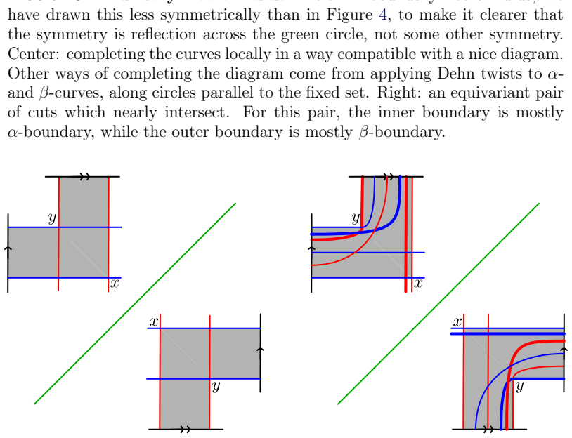
    Authors: The proof of well-definedness and invariance of the modules adapts the standard arguments from bordered Heegaard Floer homology (as in Lipshitz-Ozsváth-Thurston), with modifications to account for the action of the involution τ on the diagram and the module. No fundamentally new techniques are introduced; the key is verifying that the diagram moves and holomorphic curve counts are compatible with τ. We have revised the manuscript to explicitly state this and outline the adaptations in the construction section. revision: yes

Circularity Check

0 steps flagged

No significant circularity detected in the derivation

full rationale

The paper presents a direct constructive association of a module over the bordered Heegaard Floer algebra to an appropriate real Heegaard diagram respecting the involution τ. It then proves a gluing/pairing theorem for these modules and shows that they recover the hat variant of Guth-Manolescu real Heegaard Floer homology via gluing. The algorithm for computation on manifolds with connected fixed set follows from the existence of such diagrams and the pairing theorem. No step reduces a claimed prediction or first-principles result to a fitted parameter, self-definition, or load-bearing self-citation chain; the central objects are defined from diagrams and the invariance arguments are the standard ones adapted to the real setting, not internally forced by the paper's own inputs.

Axiom & Free-Parameter Ledger

0 free parameters · 2 axioms · 0 invented entities

The claim rests on the standard axioms of bordered Heegaard Floer theory and the real variant; no free parameters or new entities are introduced.

axioms (2)
  • standard math Heegaard diagrams represent 3-manifolds and support Floer homology constructions
    Foundational assumption of the entire Heegaard Floer program invoked throughout.
  • domain assumption The involution τ is orientation-preserving, exchanges the two boundary components, and has nonempty fixed set
    Explicit setup condition stated in the abstract for the manifolds under consideration.

pith-pipeline@v0.9.0 · 5417 in / 1404 out tokens · 60067 ms · 2026-05-09T22:56:05.353240+00:00 · methodology

discussion (0)

Sign in with ORCID, Apple, or X to comment. Anyone can read and Pith papers without signing in.

Forward citations

Cited by 1 Pith paper

Reviewed papers in the Pith corpus that reference this work. Sorted by Pith novelty score.

  1. Real link Floer homology

    math.GT 2026-04 unverdicted novelty 6.0

    Real link Floer homology is defined via real grid diagrams for symmetric links, extending real Heegaard Floer homology with combinatorial computations for over fifty small knots.

Reference graph

Works this paper leans on

41 extracted references · 20 canonical work pages · cited by 1 Pith paper

  1. [1]

    V olume II (New Delhi), Hindustan Book Agency, 2010, pp

    Denis Auroux, Fukaya categories and bordered H eegaard- F loer homology , Proceedings of the I nternational C ongress of M athematicians. V olume II (New Delhi), Hindustan Book Agency, 2010, pp. 917--941

  2. [2]

    Baker, J

    Kenneth L. Baker, J. Elisenda Grigsby, and Matthew Hedden, Grid diagrams for lens spaces and combinatorial knot F loer homology , Int. Math. Res. Not. IMRN (2008), no. 10, Art. ID rnm024, 39

  3. [3]

    Fraser Binns, Gary Guth, and Yonghan Xiao, Real sutured H eegaard F loer homology , In preparation

  4. [4]

    Irving Dai, Jennifer Hom, Matthew Stoffregen, and Linh Truong, An infinite-rank summand of the homology cobordism group, Duke Math. J. 172 (2023), no. 12, 2365--2432

  5. [5]

    Irving Dai, Sungkyung Kang, Abhishek Mallick, JungHwan Park, and Matthew Stoffregen, The (2,1) -cable of the figure-eight knot is not smoothly slice , Invent. Math. 238 (2024), no. 2, 371--390

  6. [6]

    Yakov Eliashberg, Alexander Givental, and Helmut Hofer, Introduction to symplectic field theory, Geom. Funct. Anal. (2000), no. Special Volume, Part II, 560--673, arXiv:math.SG/0010059 , GAFA 2000 (Tel Aviv, 1999)

  7. [7]

    Etnyre, Lenhard L

    John B. Etnyre, Lenhard L. Ng, and Joshua M. Sabloff, Invariants of L egendrian knots and coherent orientations , J. Symplectic Geom. 1 (2002), no. 2, 321--367

  8. [8]

    Gary Guth and Ciprian Manolescu, Real H eegaard F loer homology , 2025, arXiv:2504.09034

  9. [9]

    Gary Guth, For exotic surfaces with boundary, one stabilization is not enough, 2022, arXiv:2207.11847

  10. [10]

    Kristen Hendricks, A note on real H eegaard F loer homology and localization , 2025, arXiv:2508.03897

  11. [11]

    Reine Angew

    Matthew Hedden and Adam Simon Levine, Splicing knot complements and bordered F loer homology , J. Reine Angew. Math. 720 (2016), 129--154, arXiv:1210.7055

  12. [12]

    Kristen Hendricks and Robert Lipshitz, Involutive bordered F loer homology , Trans. Amer. Math. Soc. 372 (2019), no. 1, 389--424

  13. [13]

    Kristen Hendricks and Ciprian Manolescu, Involutive H eegaard F loer homology , Duke Math. J. 166 (2017), no. 7, 1211--1299

  14. [14]

    Sungkyung Kang, One stabilization is not enough for contractible 4-manifolds, 2022, arXiv:2210.07510

  15. [15]

    Sungkyung Kang, JungHwan Park, and Masaki Taniguchi, Exotic diffeomorphisms on a contractible 4-manifold surviving two stabilizations, 2025, arXiv:2510.12394

  16. [16]

    Jiakai Li, Monopole F loer homology and real structures , 2022, arXiv:2211.10768

  17. [17]

    Francesco Lin, A M orse- B ott approach to monopole F loer homology and the triangulation conjecture , Mem. Amer. Math. Soc. 255 (2018), no. 1221, v+162

  18. [18]

    Robert Lipshitz, A cylindrical reformulation of H eegaard F loer homology , Geom. Topol. 10 (2006), 955--1097, arXiv:math.SG/0502404

  19. [19]

    Melissa Liu, Moduli of J -holomorphic curves with L agrangian boundary conditions and open G romov- W itten invariants for an S^1 -equivariant pair , J

    C.-C. Melissa Liu, Moduli of J -holomorphic curves with L agrangian boundary conditions and open G romov- W itten invariants for an S^1 -equivariant pair , J. Iran. Math. Soc. 1 (2020), no. 1, 5--95

  20. [20]

    Jianfeng Lin and Anubhav Mukherjee, Family B auer- F uruta invariant, exotic surfaces and S male conjecture , J. Assoc. Math. Res. 3 (2025), no. 2, 237--275

  21. [21]

    Moore, Knotinfo: Table of knot invariants, URL: knotinfo.org, Current Month Current Year

    Charles Livingston and Allison H. Moore, Knotinfo: Table of knot invariants, URL: knotinfo.org, Current Month Current Year

  22. [22]

    Ozsv \'a th, and Dylan P

    Robert Lipshitz, Peter S. Ozsv \'a th, and Dylan P. Thurston, Heegaard F loer homology as morphism spaces , Quantum Topol. 2 (2011), no. 4, 381--449, arXiv:1005.1248

  23. [23]

    , Bordered F loer homology and the spectral sequence of a branched double cover I , J. Topol. 7 (2014), no. 4, 1155--1199, arXiv:1011.0499

  24. [24]

    , Computing HF by factoring mapping classes , Geom. Topol. 18 (2014), no. 5, 2547--2681, arXiv:1010.2550

  25. [25]

    , Bimodules in bordered H eegaard F loer homology , Geom. Topol. 19 (2015), no. 2, 525--724, arXiv:1003.0598

  26. [26]

    , Bordered H eegaard F loer homology , Mem. Amer. Math. Soc. 254 (2018), no. 1216, viii+279, arXiv:0810.0687

  27. [27]

    Ciprian Manolescu, Pin(2)-equivariant S eiberg- W itten F loer homology and the triangulation conjecture , J. Amer. Math. Soc. 29 (2016), no. 1, 147--176

  28. [28]

    Jin Miyazawa, A gauge theoretic invariant of embedded surfaces in 4-manifolds and exotic P^2 -knots , 2023, arXiv:2312.02041

  29. [29]

    52, American Mathematical Society, Providence, RI, 2004

    Dusa McDuff and Dietmar Salamon, J -holomorphic curves and symplectic topology , American Mathematical Society Colloquium Publications, vol. 52, American Mathematical Society, Providence, RI, 2004

  30. [30]

    Teruo Nagase, A generalization of R eidemeister- S inger theorem on H eegaard splittings , Yokohama Math. J. 27 (1979), no. 1, 23--47

  31. [31]

    Yong-Geun Oh, Fredholm theory of holomorphic discs under the perturbation of boundary conditions, Math. Z. 222 (1996), no. 3, 505--520

  32. [32]

    Peter Ozsv\'ath and Zolt\'an Szab\'o, Heegaard F loer homology and alternating knots , Geom. Topol. 7 (2003), 225--254

  33. [33]

    Ozsv \'a th and Zolt \'a n Sz ab \'o , Knot F loer homology and the four-ball genus , Geom

    Peter S. Ozsv \'a th and Zolt \'a n Sz ab \'o , Knot F loer homology and the four-ball genus , Geom. Topol. 7 (2003), 615--639, arXiv:math.GT/0301149

  34. [34]

    , Holomorphic disks and topological invariants for closed three-manifolds, Ann. of Math. (2) 159 (2004), no. 3, 1027--1158, arXiv:math.SG/0101206

  35. [35]

    , Knot F loer homology and integer surgeries , Algebr. Geom. Topol. 8 (2008), no. 1, 101--153

  36. [36]

    , Knot F loer homology and rational surgeries , Algebr. Geom. Topol. 11 (2011), no. 1, 1--68

  37. [37]

    4 (2013), no

    Ina Petkova, Cables of thin knots and bordered H eegaard F loer homology , Quantum Topol. 4 (2013), no. 4, 377--409

  38. [38]

    thesis, Harvard University, Cambridge, MA, 2003, arXiv:math.GT/0306378

    Jacob Rasmussen, Floer homology and knot complements, Ph.D. thesis, Harvard University, Cambridge, MA, 2003, arXiv:math.GT/0306378

  39. [39]

    Sucharit Sarkar and Jiajun Wang, An algorithm for computing some H eegaard F loer homologies , Ann. of Math. (2) 171 (2010), no. 2, 1213--1236, arXiv:math/0607777

  40. [40]

    Rumen Zarev, Joining and gluing sutured F loer homology , 2010, arXiv:1010.3496

  41. [41]

    Bohua Zhan, bfh \ python , https://github.com/bzhan/bfh_python