arxiv: 2604.24499 · v1 · submitted 2026-04-27 · 💻 cs.IT · math.IT· q-bio.PE· stat.AP

Recognition: unknown

Fisher Information and Dynamical Sampling I

Mattia Carrino, Stefan Hohenegger

Authors on Pith no claims yet

Pith reviewed 2026-05-08 01:19 UTC · model grok-4.3

classification 💻 cs.IT math.ITq-bio.PEstat.AP

keywords Fisher informationdynamical samplingbias calculationclusteringdegrees of freedominformation losscompartmental modeltime-series reconstruction

0 comments

The pith

Clustering degrees of freedom reduces the bias of Fisher information reconstructed from finite samples in dynamical systems.

A machine-rendered reading of the paper's core claim, the machinery that carries it, and where it could break.

The paper calculates the bias of the Fisher information for large sample sizes n when reconstructing a dynamical curve from time-series data. This bias gives a quantitative measure of how well the system's dynamics can be recovered from sampled points. The authors demonstrate that grouping or clustering the degrees of freedom lowers this bias, meaning the same data can describe the system more accurately. They also quantify the information loss due to sampling and illustrate the approach with a simple compartmental model relevant to epidemiology and other multi-variable dynamics.

Core claim

The dynamics of a system with multiple degrees of freedom can be represented as a continuous curve on a hyperplane, with the Fisher information giving the norm of infinitesimal displacements along it. From an ordered set of n sampled points, the Fisher information has a bias at large n that measures reconstruction accuracy. Clustering the degrees of freedom reduces this bias and thus the loss of information about the dynamics, allowing a quantitative estimate of how much can be reliably extracted from given data.

What carries the argument

The large-n bias of the Fisher information estimator derived from the difference between the true dynamical curve and its sampled-point approximation.

If this is right

The bias calculation supplies a concrete numerical estimate of reconstruction accuracy for any sampled time series.
Clustering reduces the bias, so the same number of samples yields a more accurate description of the clustered system.
The quantitative loss-of-information assessment sets an upper limit on how much dynamical detail can be trusted from a given dataset.
The results hold for general multi-degree-of-freedom models, not only the compartmental example.

Where Pith is reading between the lines

These are editorial extensions of the paper, not claims the author makes directly.

The same bias-reduction technique could guide experimental design when choosing how many and which variables to measure.
Analogous bias formulas might be derived for other geometric quantities defined along dynamical curves.
Testing the clustering procedure on higher-dimensional or noisy real-world datasets would check whether the large-n formula remains useful in practice.

Load-bearing premise

The large-n approximation accurately captures the bias without additional corrections from the specific model dynamics or the hyperplane geometry.

What would settle it

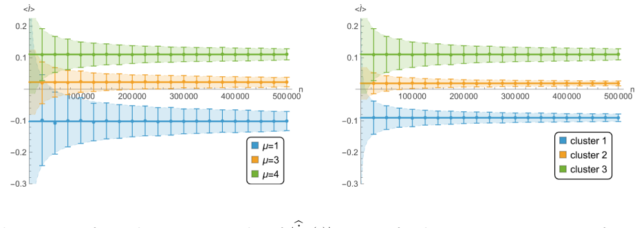
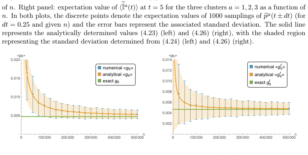
A numerical simulation of the compartmental model in which the difference between the true Fisher information (from the full curve) and the estimate from n samples converges to the predicted bias formula as n becomes large.

Figures

Figures reproduced from arXiv: 2604.24499 by Mattia Carrino, Stefan Hohenegger.

**Figure 1.** Figure 1: Left panel: Schematic representation of a probability distribution p on ∆3. Right panel: Schematic representation of a model C on ∆3. The blue vector represents the tangent vector p˙ µ to C. Geometrically, C corresponds to a curve on ∆N+1, as is schematically shown in the right panel of view at source ↗

**Figure 2.** Figure 2: Disks of same norm at different points of the simplex ∆3: each blue disk represent points with a distance ≤ √ 0.03 to the central point. review), which is well-defined in the interior of ∆N+1 (where p µ ̸= 0 ∀µ = 1, . . . , N + 1). Concretely, equation (2.9) states that the Fisher information defines the norm ds2 of the infinitesimal displacement along the curve C on the simplex ∆N+1. The tangent vector… view at source ↗

**Figure 3.** Figure 3: Schematic representation of the geometry of the dynamics: an infinitesimal displacement along the curve C is described by p˙ µdt, which is a vector of norm √gtt dt. The blue ellipse in the detail on the left indicates all ending points of vectors with norm √ gttdt (with respect ot the Shahshahani metric), but the curve C passes through only one of these points at t + dt. 8 view at source ↗

**Figure 4.** Figure 4: Schematic representation of the probabilities pb on the simplex ∆ (n) 3 for N = 2. The curve C lies on ∆3, such that the p(t) can be located anywhere on the red curve passing through the yellow triangle. The sampled probabilities pb(t) are elements of ∆ (n) 3 and are thus confined to one of the black dots. The probability that a single sampling at time t returns exactly pb(t) is given by the multinomial di… view at source ↗

**Figure 5.** Figure 5: Representation of the probability P in (2.15) on the simplex ∆3 for N = 2 and p(t) = (0.2, 0.5, 0.3) for n = 50 (left) and n = 100 (right). Points of the same colour have the same distance (measured in the Shahshahani metric) to p. Comparing the two plots shows, how the probability P becomes more and more sharply peaked around p as n is increased. 10 view at source ↗

**Figure 6.** Figure 6: Expectation value ⟨a 2 (p, p b )⟩p for N = 3 and p = (0.1, 0.2, 0.3, 0.4): the blue points show the result of a numerical computation of ⟨a 2 (p, p b )⟩p along with its standard deviation, while the orange curve represents the value in (2.18), with the shaded region representing the standard deviation. that the form of the leading term in (2.16) can be interpreted geometrically as a distance on the simp… view at source ↗

**Figure 7.** Figure 7: Schematic representation on ∆N+1 of the sampling procedure to compute the Fisher information gbtt(t). shorthand notation s µ (pb) =    2 pbµ t+ dt 2 +pbµ t− dt 2 if pb µ (t + dt 2 ) + pb µ (t − dt 2 ) ̸= 0 , 0 else (3.2) For the remainder of this work we shall assume that p(t) is in the interior of the simplex ∆N+1, such that the probability for s µ to vanish is negligibly small (at least for … view at source ↗

**Figure 8.** Figure 8: Illustration of the clustering according to the change of information I˙ µ : for fixed t, the black dots represent the values I˙ µ (t) for µ = 1, . . . , N + 1. The clustering groups degrees of freedom with ’similar’ I˙ µ (t) into the clusters Aa for a = 1, . . . , ℓ. Indeed, the change of the Fisher information (4.6) can equivalently be written in the form ∆gtt = N X +1 µ=1 p µ I˙ µ − ˙I f(µ) 2 , (4.8)… view at source ↗

**Figure 9.** Figure 9: Illustration of the variance of the couplings over all clusters. The change in the Fisher information is the expectation value over the variances (4.14) of the couplings d µ over all clusters. Before closing this Subsection, we remark that (4.13) (with (4.14)) depends on the couplings, which is primarily of conceptual interest, since it links the loss of information due to clustering to the couplings d µ .… view at source ↗

**Figure 10.** Figure 10: Left panel: numerical choice of the transmission and recovery rates for N + 1 = 10 pathogens. We shall use this choice for all numerical results in the remainder of this Section. Right panel: the probabilities p µ (t) that constitute the statistical model C in (5.2) as functions of time. They have been obtained as numerical solutions from (5.1) using a Runge-Kutta formalism, with γ µ and ϵ µ as shown in t… view at source ↗

**Figure 11.** Figure 11: The expectation value ⟨d⟩p (5.3) as a function of time for the numerical solutions found in view at source ↗

**Figure 12.** Figure 12: Left panel: time derivative of the self-information I˙ µ for each of the N + 1 = 10 variants as functions of time. Variants showing a similar I˙ µ are combined into a cluster, which is indicated by the shaded regions: cluster 1 (blue): µ ∈ A1 = {1, 2, 5, 8, 9}, cluster 2 (orange): µ ∈ A2 = {3, 6, 7, 10}, cluster 3 (green): µ ∈ A3 = {4}. Right panel: Fisher information gtt(t) (blue curve) (2.6) for the mod… view at source ↗

**Figure 13.** Figure 13: Left panel: expectation value of ⟨I b˙ µ (t)⟩ at t = 5 for the variants µ = 1, 3, 4 as a function of n. Right panel: expectation value of ⟨ b˙I a (t)⟩ at t = 5 for the three clusters a = 1, 2, 3 as a function of n. In both plots, the discrete points denote the expectation values of 1000 samplings of pb µ (t ± dt) (for dt = 0.25 and given n) and the error bars represent the associated standard deviation. T… view at source ↗

**Figure 14.** Figure 14: Left panel: expectation value of the Fisher information ⟨gbtt(t)⟩ in (3.1) at t = 5 as a function of n. Right panel: expectation value of the Fisher information ⟨gb f tt(t)⟩ in (4.17) for the clustered system at t = 5 as a function of n. In both plots, the discrete points denote the expectation values of 500 samplings of pb µ (t ± dt) (for dt = 0.25 and given n) and the error bars represent the associated… view at source ↗

**Figure 15.** Figure 15: Left panel: expectation value of the Fisher information ⟨gbtt(t)⟩ in (3.1) for n = 100.000 as a function of t. Right panel: expectation value of the Fisher information ⟨gb f tt(t)⟩ in (4.17) for the clustered system for n = 100.000 as a function of t. In both plots, the discrete points denote the expectation values of 500 samplings of pb µ (t ± dt) (for dt = 0.25) and the error bars represent the associat… view at source ↗

**Figure 16.** Figure 16: Left panel: comparison of the change of information I b˙ µ (solid points) obtained from a single sampling of C with the exact value I˙ µ (solid line) for three variants. The error bars indicate the standard deviation as in (4.22). As is evident, for certain times t, the theoretical value of I˙ µ lies outside of the range set by the latter. Right panel: same comparison after Gaussian filtering of Cb with t… view at source ↗

**Figure 17.** Figure 17: Left panel: comparison between gtt(t) and g f tt(t) (for several ℓ) obtained from a SIR model with N + 1 = 50. Increasing the number of clusters ℓ generally decreases ∆gtt. Right panel: difference −∆gtt = g f tt − gtt over ℓ obtained from the Fisher information in the left panel for t = 1. We find an elbow for this curve at ℓ ∗ = 6, thus providing a strategy to find the value for ℓ that maximises the perf… view at source ↗

read the original abstract

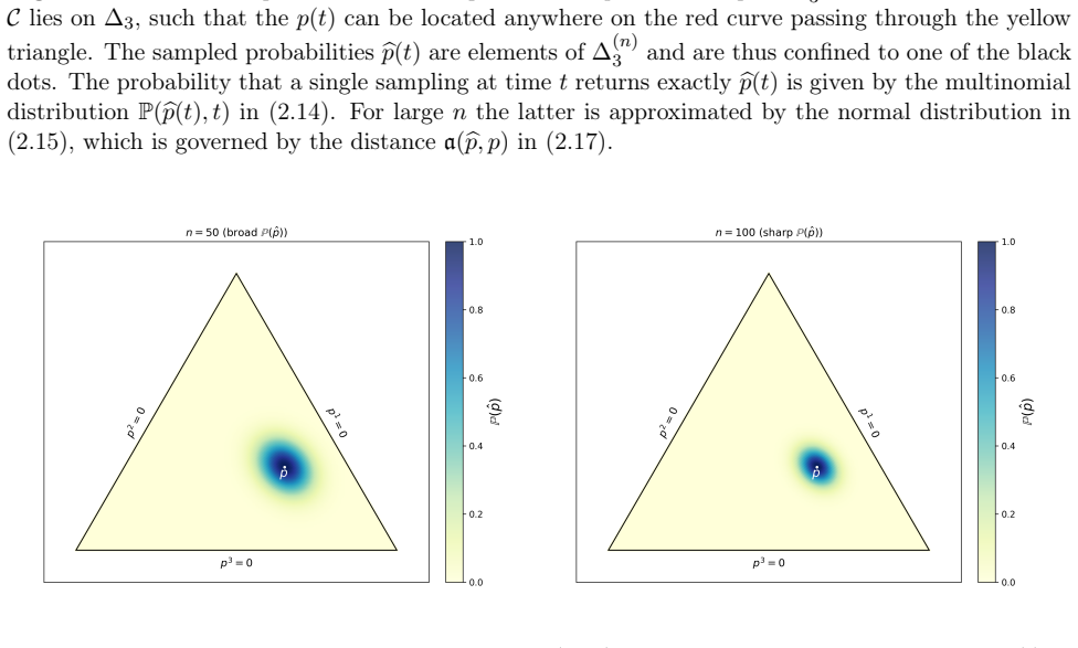
Information theory is a powerful framework to capture aspects of dynamical systems with multiple degrees of freedom. Mathematically, the dynamics can be represented as a continuous curve $\mathcal{C}$ on a suitable hyperplane in flat space and the Fisher information provides the norm of an infinitesimal displacement along this curve. In many applications, however, we do not have direct access to $\mathcal{C}$. Instead, we have to reconstruct the latter from a time-series of measurements (obtained as samples of size $n$), which are represented by an ordered set of points $\widehat{\mathcal{C}}$ on the same hyperplane. In this work, we calculate the bias of the Fisher information for large $n$, which provides a quantitative estimation for how accurately the dynamics of a system can be reconstructed from a given set of sampled data. Based on this result, we show that a clustering of the degrees of freedom reduces the bias and thus improves the accuracy with which the new system can be described with the same data. Inspired by a recent proposal for such a clustering, we provide a quantitive assessment of the loss of information, which allows to estimate how much information about the dynamics of a system can reliably be extracted based on a given set of data. We illustrate our findings in the case of a simple compartmental model. Although the latter is inspired by epidemiology, the results of this work are applicable to very general dynamical models with multiple degrees of freedom.

Editorial analysis

A structured set of objections, weighed in public.

Desk editor's note, referee report, simulated authors' rebuttal, and a circularity audit. Tearing a paper down is the easy half of reading it; the pith above is the substance, this is the friction.

Desk Editor's Note private letter to a colleague

They derive an explicit large-n bias for Fisher information on sampled dynamical curves and claim clustering reduces it, but the parametrization may need extra terms.

read the letter

The punchline here is that the authors calculate the bias of the Fisher information for large n in reconstructing a dynamical curve from samples, and then demonstrate that clustering the degrees of freedom reduces this bias. They represent the dynamics as a continuous curve on a hyperplane, with time-series data as points on an estimated curve. The Fisher information serves as the norm for small displacements. From this they derive the bias in the large-n limit, giving a way to estimate reconstruction accuracy. They extend this to show clustering helps, and quantify the information loss, with an example in a compartmental model inspired by epidemiology. This is new relative to the cited work: the specific bias formula tied to the sampling and the quantitative clustering assessment. The paper does well in providing a clear application to a simple model, making the general claims more tangible for readers in applied fields like biology or physics. The main soft spot is around the large-n approximation. The points are ordered along the curve, so the sampling is not i.i.d. from a fixed distribution but follows the time parametrization. If the bias derivation does not keep terms that depend on the curve speed or local density, then the predicted improvement from clustering could be off, since clustering changes the effective dimension and the measure on the reduced space. The abstract presents the approximation as holding without extra corrections, which is the part that needs close checking in the full derivation. The rest of the setup uses standard information geometry, and there is no sign of circularity in the bias calculation itself. The reference to the recent clustering proposal is handled separately. This paper is for researchers working on information-theoretic tools for multi-variable dynamical systems who want quantitative estimates of sampling effects. A reader focused on applied modeling would find the formula and example useful. It has a solid enough core calculation to merit a serious referee, mainly to verify the bias steps and the handling of the curve parametrization. I would recommend sending it to peer review.

Referee Report

2 major / 3 minor

Summary. The paper models dynamical systems as continuous curves C on a hyperplane in flat space, with time-series data as ordered samples forming a reconstruction Ĉ. It derives the large-n bias of the Fisher information (providing a quantitative measure of reconstruction accuracy for the dynamics) and shows that clustering degrees of freedom reduces this bias, improving accuracy with the same data. A quantitative assessment of information loss is given, inspired by a recent clustering proposal, and illustrated via a simple compartmental model.

Significance. If the large-n bias derivation is complete and accounts for the curve parametrization, the work supplies a concrete information-theoretic tool for assessing finite-sample accuracy in reconstructing multi-degree-of-freedom dynamics, with the clustering result offering a practical route to bias reduction. The compartmental-model illustration suggests applicability to epidemiology and similar systems, but the overall significance depends on verifying that the bias formula retains all relevant sampling-measure corrections.

major comments (2)

[Bias calculation] Bias calculation (derivation of large-n Fisher bias): the central claim relies on an explicit asymptotic bias formula for Fisher information computed from ordered points on Ĉ. Standard i.i.d. asymptotic expansions do not automatically apply because the samples are the push-forward of the time parametrization along C; the derivation must retain terms proportional to local sampling density and curve speed ||dC/dt||. If these velocity- or density-dependent corrections are omitted, the subsequent claim that clustering reduces bias cannot be guaranteed, since clustering simultaneously lowers dimension and alters the induced measure on the reduced hyperplane. Please state the precise bias expression (including any omitted terms) and confirm whether the large-n limit is taken with fixed parametrization speed.
[Clustering assessment] Clustering and information-loss assessment: the quantitative statement that clustering reduces bias and improves accuracy is load-bearing for the paper's second main result, yet it is not shown by direct substitution into the derived bias formula. The assessment references an external recent proposal but does not exhibit how the bias term scales with the number of clustered degrees of freedom or with the modified sampling measure. An explicit calculation linking the two would be required to support the claim.

minor comments (3)

[Abstract] The abstract refers to 'a recent proposal for such a clustering' without a citation; add the reference in both the abstract and the main text.
[Compartmental model] In the compartmental-model illustration, the construction of the curve C from the model equations, the choice of time parametrization, and the numerical values of n and parameters are not fully specified; these details are needed for reproducibility of the bias and clustering results.
[Notation] Notation for the reconstructed curve (Ĉ) and the hyperplane embedding should be introduced once and used consistently; occasional shifts between C and Ĉ in the text can be clarified.

Simulated Author's Rebuttal

2 responses · 0 unresolved

We thank the referee for the careful reading of our manuscript and the constructive comments, which have helped us clarify key aspects of the derivation and strengthen the presentation. We address each major comment point by point below. Where revisions are needed to make the bias formula and clustering analysis fully explicit, we have incorporated them into the revised version.

read point-by-point responses

Referee: [Bias calculation] Bias calculation (derivation of large-n Fisher bias): the central claim relies on an explicit asymptotic bias formula for Fisher information computed from ordered points on Ĉ. Standard i.i.d. asymptotic expansions do not automatically apply because the samples are the push-forward of the time parametrization along C; the derivation must retain terms proportional to local sampling density and curve speed ||dC/dt||. If these velocity- or density-dependent corrections are omitted, the subsequent claim that clustering reduces bias cannot be guaranteed, since clustering simultaneously lowers dimension and alters the induced measure on the reduced hyperplane. Please state the precise bias expression (including any omitted terms) and confirm whether the large-n limit is taken with fixed parametrization speed.

Authors: We appreciate this observation on the non-i.i.d. character of the sampling. In the original derivation (Section 3), the bias is obtained from the push-forward of the uniform time measure along the curve C, so the leading large-n bias term already incorporates the local sampling density ρ(t) and the speed ||dC/dt|| through the Jacobian factor that maps the time parametrization to the hyperplane measure. The precise expression is Bias(Î) = (1/n) ∫ [ρ(t) / ||dC/dt||] · Tr(∇² log p) dt + O(1/n²), where the integral is over the fixed time interval. The large-n limit is taken with parametrization speed held fixed (i.e., fixed total observation time T and n → ∞). To eliminate any ambiguity we have now inserted the full expanded formula, including the velocity- and density-dependent corrections, as Equation (12) in the revised manuscript. This explicit form confirms that the subsequent clustering analysis remains valid. revision: yes
Referee: [Clustering assessment] Clustering and information-loss assessment: the quantitative statement that clustering reduces bias and improves accuracy is load-bearing for the paper's second main result, yet it is not shown by direct substitution into the derived bias formula. The assessment references an external recent proposal but does not exhibit how the bias term scales with the number of clustered degrees of freedom or with the modified sampling measure. An explicit calculation linking the two would be required to support the claim.

Authors: We agree that a direct substitution strengthens the argument. In the revised Section 4 we substitute the reduced dimension k < d into the bias formula derived above. The leading bias term scales as k/d times the original bias, while the change in the induced sampling measure on the clustered hyperplane contributes only an O(1/n) correction that is sub-dominant to the bias reduction. We have added this explicit scaling calculation together with a short numerical check on the compartmental model; the information-loss estimate is thereby tied directly to the bias expression rather than relying solely on the external reference. revision: yes

Circularity Check

0 steps flagged

No circularity: bias derivation uses standard asymptotic expansion independent of clustering result

full rationale

The paper computes the large-n bias of the Fisher information directly from the geometry of ordered samples on the reconstructed curve Ĉ, applying standard information-geometric asymptotics to the push-forward measure induced by the time parametrization. This bias formula is then applied to demonstrate that clustering reduces the bias. No equation equates the target quantity to a fitted parameter or to a self-citation; the clustering reference is explicitly to an external recent proposal. The central claim therefore rests on an independent derivation rather than on any self-definitional, fitted-input, or load-bearing self-citation step.

Axiom & Free-Parameter Ledger

0 free parameters · 2 axioms · 0 invented entities

The work rests on standard information-theoretic representations of dynamics and a large-n limit; no free parameters or new entities are introduced in the abstract.

axioms (2)

domain assumption Dynamics represented as continuous curve C on hyperplane in flat space with Fisher information as norm of displacement.
Invoked to define the mathematical setup for sampling and bias.
domain assumption Large-n approximation suffices to compute the bias of the Fisher information estimator.
Central to the quantitative estimation result.

pith-pipeline@v0.9.0 · 5554 in / 1416 out tokens · 78477 ms · 2026-05-08T01:19:23.800111+00:00 · methodology

discussion (0)

Reference graph

Works this paper leans on

92 extracted references · 2 canonical work pages

[1]

Information clustering and pathogen evolution,

B. Filoche and S. Hohenegger, “Information clustering and pathogen evolution,”Physica A: Statistical Mechanics and its Applications, vol. 672, p. 130647, 2025

2025
[2]

On the mathematical foundations of theoretical statistics,

R. A. Fisher and E. J. Russell, “On the mathematical foundations of theoretical statistics,” Philosophical Transactions of the Royal Society of London. Series A, Containing Papers of a Mathematical or Physical Character, vol. 222, no. 594-604, pp. 309–368, 1922

1922
[3]

A mathematical theory of communication,

C. E. Shannon, “A mathematical theory of communication,”The Bell System Technical Journal, vol. 27, no. 3, pp. 379–423, 1948

1948
[4]

Shannon and W

C. Shannon and W. Weaver,The mathematical theory of communication. University of Illinois Press, 1949

1949
[5]

Spaces of statistical parameters,

H. Hotelling, “Spaces of statistical parameters,”Bulletin of the American Mathematical Society (AMS), vol. 36, p. 191, 1930

1930
[6]

Information and the accuracy attainable in the estimation of statistical pa- rameters,

R. C. Rao, “Information and the accuracy attainable in the estimation of statistical pa- rameters,”Bulletin of the Calcutta Mathematical Society, vol. 37, pp. 81–91, 1945

1945
[7]

Badii and A

R. Badii and A. Politi,Complexity: Hierarchical Structures and Scaling in Physics. Cam- bridge Nonlinear Science Series, Cambridge University Press, 1997

1997
[8]

Castiglione, M

P. Castiglione, M. Falcioni, A. Lesne, and A. Vulpiani,Chaos and Coarse Graining in Statistical Mechanics. Cambridge University Press, 2008

2008
[9]

Two inequalities implied by unique decipherability,

B. McMillan, “Two inequalities implied by unique decipherability,”IRE Transactions on Information Theory, vol. 2, no. 4, pp. 115–116, 1956

1956
[10]

A method for the construction of minimum-redundancy codes,

D. A. Huffman, “A method for the construction of minimum-redundancy codes,”Proceed- ings of the IRE, vol. 40, no. 9, pp. 1098–1101, 1952

1952
[11]

Goldman,Information Theory

S. Goldman,Information Theory. Prentice-Hall (University of Michigan), 1953. Prentice- Hall electrical engineering series

1953
[12]

Shannon entropy: a rigorous notion at the crossroads between probability, information theory, dynamical systems and statistical physics,

A. Lesne, “Shannon entropy: a rigorous notion at the crossroads between probability, information theory, dynamical systems and statistical physics,”Mathematical Structures in Computer Science, vol. 24, no. 3, p. e240311, 2014

2014
[13]

Information theory and statistical mechanics,

E. T. Jaynes, “Information theory and statistical mechanics,”Phys. Rev., vol. 106, pp. 620– 630, May 1957. 36

1957
[14]

Information theory and statistical mechanics. ii,

E. T. Jaynes, “Information theory and statistical mechanics. ii,”Phys. Rev., vol. 108, pp. 171–190, Oct 1957

1957
[15]

The large deviation approach to statistical mechanics,

H. Touchette, “The large deviation approach to statistical mechanics,”Physics Reports, vol. 478, p. 1–69, July 2009

2009
[16]

Statistical manifolds,

S. L. Lauritzen, “Statistical manifolds,”Differential geometry in statistical inference, vol. 10, pp. 163–216, 1987

1987
[17]

An invariant form for the prior probability in estimation problems,

H. Jeffreys, “An invariant form for the prior probability in estimation problems,”Proc. R. Soc. Lond. A, vol. 186(1007), pp. 453–461, 1946

1946
[18]

Translationsofmathematical monographs, American Mathematical Society, 2000

S.AmariandH.Nagaoka,Methods of Information Geometry. Translationsofmathematical monographs, American Mathematical Society, 2000

2000
[19]

Differential Geometry of Curved Exponential Families-Curvatures and Infor- mation Loss,

S.-I. Amari, “Differential Geometry of Curved Exponential Families-Curvatures and Infor- mation Loss,”The Annals of Statistics, vol. 10, no. 2, pp. 357 – 385, 1982

1982
[20]

Differential Geometry in Statistical Inference,

S. Amari, O. E. Barndorff-Nielsen, R. E. Kass, S. L. Lauritzen, and C. R. Rao, “Differential Geometry in Statistical Inference,”Lecture Notes-Monograph Series, vol. 10, pp. i – 240
[21]

T. M. Cover and J. A. Thomas,Elements of Information Theory. John Wiley & Sons, Inc., 2006. second edition

2006
[22]

A mathematical examination of the methods of determining the accuracy of observation by the mean error, and by the mean square error,

R. A. Fisher, “A mathematical examination of the methods of determining the accuracy of observation by the mean error, and by the mean square error,”Monthly Notices of the Royal Astronomical Society, vol. 80, pp. 758–770, 06 1920

1920
[23]

Shahshahani,A new mathematical framework for the study of linkage and selection

S. Shahshahani,A new mathematical framework for the study of linkage and selection. Memoirs of the American Mathematical Society ; number 211, American Mathematical Society (Providence), 1st ed. ed., 1979 - 1979

1979
[24]

On the change of population fitness by natural selection,

M. Kimura, “On the change of population fitness by natural selection,”Heredity, vol. 12, p. 45–167, 1958

1958
[25]

Information geometry and evolutionary game theory,

M. Harper, “Information geometry and evolutionary game theory,” 2009. arXiv/0911.1383

work page arXiv 2009
[26]

The projection dynamic and the replicator dynamic,

W. H. Sandholm, E. Dokumacı, and R. Lahkar, “The projection dynamic and the replicator dynamic,”Games and Economic Behavior, vol. 64, no. 2, pp. 666–683, 2008. Special Issue in Honor of Michael B. Maschler

2008
[27]

W. H. Sandholm,Population games and evolutionary dynamics / William H. Sandholm. Economic learning and social evolution, Cambridge, Mass: MIT Press, 1st ed. ed., 2010

2010
[28]

Riemannian game dynamics,

P. Mertikopoulos and W. H. Sandholm, “Riemannian game dynamics,”Journal of Eco- nomic Theory, vol. 177, pp. 315–364, 2018

2018
[29]

Hofbauer and K

J. Hofbauer and K. Sigmund,Evolutionary Games and Population Dynamics. Cambridge University Press, 1998

1998
[30]

Information theory unification of epidemio- logical and population dynamics,

B. Filoche, S. Hohenegger, and F. Sannino, “Information theory unification of epidemio- logical and population dynamics,”Physica A, vol. 650, p. 129970, 2024. 37

2024
[31]

The method of types [information theory],

I. Csiszar, “The method of types [information theory],”IEEE Transactions on Information Theory, vol. 44, no. 6, pp. 2505–2523, 1998

1998
[32]

Csiszár and J

I. Csiszár and J. Körner,Information Theory: Coding Theorems for Discrete Memoryless Systems. Cambridge University Press, 2 ed., 2011

2011
[33]

The source coding theorem revisited: A combinatorial approach,

G. Longo and A. Sgarro, “The source coding theorem revisited: A combinatorial approach,” IEEE Transactions on Information Theory, vol. 25, no. 5, pp. 544–548, 1979

1979
[34]

Asymptotically optimal tests for multinomial distributions,

W. Hoeffding, “Asymptotically optimal tests for multinomial distributions,”The Annals of Mathematical Statistics, vol. 36, no. 2, pp. 369–401, 1965

1965
[35]

Dembo and O

A. Dembo and O. Zeitouni,Large Deviations Techniques and Applications. Springer, 2 ed., 2009

2009
[36]

Bender and S

C. Bender and S. Orszag,Advanced Mathematical Methods for Scientists and Engineers I: Asymptotic Methods and Perturbation Theory. Springer, 01 1978

1978
[37]

Fisher Information and Dynamical Sampling II,

M. Carrino and S. Hohenegger, “Fisher Information and Dynamical Sampling II,”in prepa- ration
[38]

Applications of mathematics to medical problems,

A. McKendrick, “Applications of mathematics to medical problems,”Proc. Edinburgh Math. Soc., vol. 44, pp. 98–130, 1926

1926
[39]

A contribution to the mathematical theory of epidemics,

W. O. Kermack, A. McKendrick, and G. T. Walker, “A contribution to the mathematical theory of epidemics,”Proceedings of the Royal Society A, vol. 115, pp. 700–721, 1927

1927
[40]

Entropy differential metric, distance and divergence measures in probability spaces: A unified approach,

J. Burbea and C. Rao, “Entropy differential metric, distance and divergence measures in probability spaces: A unified approach,”Journal of Multivariate Analysis, vol. 12, no. 4, pp. 575–596, 1982

1982
[41]

An elementary introduction to information geometry,

F. Nielsen, “An elementary introduction to information geometry,”Entropy, vol. 22, no. 10, 2020

2020
[42]

On Information and Sufficiency,

S. Kullback and R. A. Leibler, “On Information and Sufficiency,”The Annals of Mathe- matical Statistics, vol. 22, no. 1, pp. 79 – 86, 1951

1951
[43]

Information-type measures of differences of probability distributions and indi- rect observations,

I. Csiszár, “Information-type measures of differences of probability distributions and indi- rect observations,”Studia Sci. Math. Hungarica, vol. 2, pp. 299 – 318, 1967

1967
[44]

On topological properties off-divergence,

I. Csiszár, “On topological properties off-divergence,”Studia Sci. Math. Hungarica, vol. 2, pp. 329 – 339, 1967

1967
[45]

A foundation of information geometry,

S.-I. Amari, “A foundation of information geometry,”Electronics and Communications in Japan (Part I: Communications), vol. 66, no. 6, pp. 1–10, 1983

1983
[46]

Schervish,Theory of statistics

M. Schervish,Theory of statistics. Springer-Verlag, 1995

1995
[47]

Reading a neural code,

W. Bialek, F. Rieke, R. R. de Ruyter van Steveninck, and D. Warland, “Reading a neural code,”Science, vol. 252, no. 5014, pp. 1854–1857, 1991. 38

1991
[48]

Entropy and information in neural spike trains,

S. P. Strong, R. Koberle, R. R. de Ruyter van Steveninck, and W. Bialek, “Entropy and information in neural spike trains,”Phys. Rev. Lett., vol. 80, pp. 197–200, Jan 1998

1998
[49]

Binless strategies for estimation of information from neural data,

J. D. Victor, “Binless strategies for estimation of information from neural data,”Phys. Rev. E, vol. 66, p. 051903, Nov 2002

2002
[50]

Nonparametric entropy estimation. an overview,

J. Beirlant, E. J. Dudewicz, L. Györfi, and I. Denes, “Nonparametric entropy estimation. an overview,” 1997

1997
[51]

Grenander,Abstract inference

U. Grenander,Abstract inference. Wiley, 1981

1981
[52]

On a statistical estimate for the entropy of a sequence of independent random variables,

G. P. Basharin, “On a statistical estimate for the entropy of a sequence of independent random variables,”Theory of Probability & Its Applications, vol. 4, no. 3, pp. 333–336, 1959

1959
[53]

Estimation of entropy and mutual information,

L. Paninski, “Estimation of entropy and mutual information,”Neural Computation, vol. 15, pp. 1191–1253, 06 2003

2003
[54]

Age-incidence in relation with cycles of disease prevalence,

W. Hamer, “Age-incidence in relation with cycles of disease prevalence,”Trans. Epi- dem. Soc. London, vol. 15, pp. 64–77, 1896
[55]

Epidemic disease in England: The evidence of variability and of persistency of type; Lecture 1,

W. Hamer, “Epidemic disease in England: The evidence of variability and of persistency of type; Lecture 1,”Lancet, pp. 569–574, March 1906

1906
[56]

Epidemic disease in England: The evidence of variability and of persistency of type; Lecture 2,

W. Hamer, “Epidemic disease in England: The evidence of variability and of persistency of type; Lecture 2,”Lancet, pp. 655–662, March 1906

1906
[57]

Epidemic disease in England: The evidence of variability and of persistency of type; Lecture 3,

W. Hamer, “Epidemic disease in England: The evidence of variability and of persistency of type; Lecture 3,”Lancet, pp. 733–739, March 1906

1906
[58]

The Prevention of Malaria,

R. Ross, “The Prevention of Malaria,”second edition, John Murray, London, 1911

1911
[59]

An application of the theory of probabilities to the study ofa prioripathometry: Part I,

R. Ross, “An application of the theory of probabilities to the study ofa prioripathometry: Part I,”Proc. Roy. Soc. Lond. A, vol. 92, pp. 204–230, 1916

1916
[60]

An application of the theory of probabilities to the study ofa prioripathometry: Part II,

R. Ross and H. Hudson, “An application of the theory of probabilities to the study ofa prioripathometry: Part II,”Proc. Roy. Soc. Lond. A, vol. 93, pp. 212–225, 1916

1916
[61]

An application of the theory of probabilities to the study ofa prioripathometry: Part III,

R. Ross and H. Hudson, “An application of the theory of probabilities to the study ofa prioripathometry: Part III,”Proc. Roy. Soc. Lond. A, vol. 93, pp. 225–240, 1916

1916
[62]

The rise and fall of epidemics,

A. McKendrick, “The rise and fall of epidemics,”Paludism (Transactions of the Committee for the Study of Malaria in India), vol. 1, pp. 54–66, 1912

1912
[63]

Studies on the theory of continuous probabilities, with special reference to its bearing on natural phenomena of a progressive nature,

A. McKendrick, “Studies on the theory of continuous probabilities, with special reference to its bearing on natural phenomena of a progressive nature,”Proceedings of the London Mathematical Society, vol. 13, pp. 401–416, 1914

1914
[64]

R. M. Anderson and R. M. May,Infectious Diseases of Humans: Dynamics and Control. Oxford University Press, 05 1991. 39

1991
[65]

Brauer, C

F. Brauer, C. Castillo-Chavez, and Z. Feng,Mathematical Models in Epidemiology, vol. 69, Springer, New York. Texts in Applied Mathematics, 2019

2019
[66]

Brauer, P

F. Brauer, P. Driessche, and J. Wu,Mathematical Epidemiology, vol. 1945, Lecture Notes in Mathematics, Mathematical Biosciences Subseries. Springer Berlin, Heidelberg, 2008. ISBN: 978-3-540-78911-6

1945
[67]

Capasso,Mathematical Structures of Epidemic Systems

V. Capasso,Mathematical Structures of Epidemic Systems. Springer Berlin, 1993. ISBN: 978-3-540-70514-7

1993
[68]

Diekmann and J

O. Diekmann and J. A. P. Heesterbeek,Mathematical Epidemiology of Infectious Diseases. John Wiley & Sons, Chichester, 2000

2000
[69]

Prince- ton University Press, 2008

M.J.KeelingandP.Rohani,Modeling Infectious Diseases in Humans and Animals. Prince- ton University Press, 2008. ISBN: 9780691116174

2008
[70]

Martcheva,An Introduction to Mathematical Epidemiology, vol

M. Martcheva,An Introduction to Mathematical Epidemiology, vol. 61, Texts in Applied Mathematics. Springer New York, NY, 2015. ISBN: 978-1-4899-7612-3

2015
[71]

The field theoretical ABC of epidemic dynamics,

G. Cacciapaglia, C. Cot, M. D. Morte, S. Hohenegger, F. Sannino, and S. Vatani, “The field theoretical ABC of epidemic dynamics,” [arXiv 2101.11399 [q-bio.PE]

work page arXiv
[72]

Sur la division des corps matériels en parties,

H. Steinhaus, “Sur la division des corps matériels en parties,”Bull. Acad. Polon. Sci. Cl. III., vol. 4, pp. 801–804, 1956

1956
[73]

Some methods for classification and analysis of multivariate observations,

J. MacQueen, “Some methods for classification and analysis of multivariate observations,” inProc. Fifth Berkeley Sympos. Math. Statist. and Probability (Berkeley, Calif., 1965/66), Vol. I: Statistics, pp. 281–297, Univ. California Press, Berkeley, CA, 1967

1965
[74]

Least squares quantization in pcm,

S. Lloyd, “Least squares quantization in pcm,”IEEE Transactions on Information Theory, vol. 28, no. 2, pp. 129–137, 1982

1982
[75]

Cluster analysis of multivariate data: efficiency versus interpretability of classifications,

E. W. Forgy, “Cluster analysis of multivariate data: efficiency versus interpretability of classifications,”Biometrics, vol. 21, no. 3, pp. 768–769, 1965

1965
[76]

The jackknife-a review,

R. G. Miller, “The jackknife-a review,”Biometrika, vol. 61, pp. 1–15, 04 1974

1974
[77]

Bootstrap: More than a stab in the dark?,

G. A. Young, “Bootstrap: More than a stab in the dark?,”Statistical Science, vol. 9, no. 3, pp. 382–395, 1994

1994
[78]

Feller,An Introduction to Probability Theory and Its Applications, vol I.Wiley, 3 ed., 1957

W. Feller,An Introduction to Probability Theory and Its Applications, vol I.Wiley, 3 ed., 1957

1957
[79]

Feller,An Introduction to Probability Theory and Its Applications, vol II.Wiley, 2 ed., 1957

W. Feller,An Introduction to Probability Theory and Its Applications, vol II.Wiley, 2 ed., 1957

1957
[80]

Wasserman,All of statistics: a concise course in statistical inference

L. Wasserman,All of statistics: a concise course in statistical inference. New York: Springer, 2010

2010

Showing first 80 references.