arxiv: 2604.27260 · v1 · submitted 2026-04-29 · 🧮 math.MG · math.CO· math.OC

Recognition: unknown

Exact Flatness Constant for One-Point Convex Bodies and the Discrete Isominwidth Problem: The Planar Case

Ansgar Freyer, Gennadiy Averkov, Giulia Codenotti, Kyle Huang

Pith reviewed 2026-05-07 10:24 UTC · model grok-4.3

classification 🧮 math.MG math.COmath.OC

keywords flatness constantlattice widthconvex bodiesinterior lattice pointsisominwidth inequalityplanar geometry

0 comments

The pith

Any planar convex body with at most one interior lattice point has lattice width at most 3.

A machine-rendered reading of the paper's core claim, the machinery that carries it, and where it could break.

The paper proves that the flatness constant Flt(2,1) equals exactly 3. This means every convex body in the plane that contains at most one lattice point in its interior cannot exceed lattice width 3. The result settles the exact maximum width for such bodies and produces an isominwidth inequality that relates the number of lattice points inside a planar convex body to its directional widths. A reader would care because the bound limits how large a convex set can grow in a direction while still avoiding most lattice points, with direct ties to counting problems and optimization over integer grids.

Core claim

The authors show that Flt(2,1) = 3. Every convex body in R^2 with at most one interior lattice point therefore has lattice width at most 3, and this value is tight. The proof combines supporting-line arguments with enumeration of possible interior-point configurations to obtain both the upper bound and matching examples.

What carries the argument

The flatness constant Flt(d,k), the supremum of lattice widths taken over all convex bodies in R^d that contain at most k interior lattice points.

If this is right

The exact value yields an isominwidth inequality that bounds the lattice-point enumerator of any planar convex body from below by a function of its isominwidth.
It confirms the planar case of the discrete isominwidth problem.
It supplies the missing exact constant needed to relate the classical flatness problem to Makai's conjectural dual form of Minkowski's theorem.

Where Pith is reading between the lines

These are editorial extensions of the paper, not claims the author makes directly.

The width bound could be used to restrict the feasible region in 2D integer linear programs before enumeration.
The same geometric technique might determine Flt(3,1) or the value for other small k in the plane.
It constrains the possible areas and shapes of convex bodies that are nearly lattice-point free.

Load-bearing premise

Convex bodies are closed sets in the plane and the lattice is the standard integer lattice Z^2, with width measured as the minimum distance between parallel supporting lines.

What would settle it

A single closed convex set in the plane that contains at most one interior integer point yet has lattice width 4 or greater would disprove the equality.

Figures

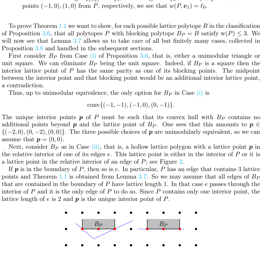
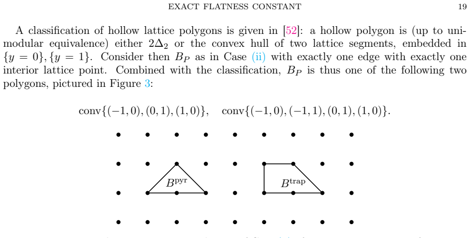
Figures reproduced from arXiv: 2604.27260 by Ansgar Freyer, Gennadiy Averkov, Giulia Codenotti, Kyle Huang.

**Figure 1.** Figure 1: The edges f(−1) and f1, emanating from f0. As they separate the points (−1, 0),(1, 0) from P, respectively, we see that w(P, e1) = ℓ0. To prove Theorem 1.1 we want to show, for each possible lattice polytope B in the classification of Proposition 3.6, that all polytopes P with blocking polytope BP = B satisfy w(P) ≤ 3. We will now see that Lemma 3.7 allows us to take care of all but finitely many cases, co… view at source ↗

**Figure 2.** Figure 2: When BP has three colinear boundary points (visualized in red), either the inside point is an interior lattice point of P, as on the left, or all three points lie on an edge of P, as on the right. In this situation Lemma 3.7 applies view at source ↗

**Figure 3.** Figure 3: The two remaining polygons of Case (ii) of Proposition 3.6. We refer to them as Bpyr and Btrap, respectively. Now consider BP as in Case (iii). There are 16 lattice polygons (up to unimodular transformation) with one interior lattice point, see [52]. By Lemma 3.7, we can assume that BP has no edge of lattice length greater than 1. Filtering the list of the 16 so accordingly yields the following 5 polygons… view at source ↗

**Figure 4.** Figure 4: The 5 remaining polygons of Case (iii) of Proposition 3.6. We refer to them as Bterm, Bkite , Bcross , Bpent , and Bhex, respectively. Compare with view at source ↗

**Figure 5.** Figure 5: The configuration as in Lemma 3.9. The regions S1, ..., S6 are as labeled, in blue. Observe that the points p1 , p6 must lie between the lines {y − x = −1} and {y − x = 1}, and that p1 , p6 and (−1, −1) are colinear: that is, there exists λ ≥ 0 such that p1 , p6 lie on the line {y + 1 = −λ(x + 1)}. We then see that p1,y + p6,x is minimized if p1 , p6 lie respectively on lines {y − x = −1}, {y − x = 1}, in … view at source ↗

**Figure 6.** Figure 6: The regions as in Lemma 3.11. The regions S1, ..., S5 are as labeled, in blue. Proof. We apply Lemma 3.4, and further cut out σ(1,1) to obtain S3. □ Lemma 3.12. Let P be a 1-maximal polygon such that BP = Bpent. Then w(P) < 3. Proof. Let pi , 1 ≤ i ≤ 5, be (possibly degenerate) vertices of P in the regions Si of Lemma 3.11, respectively. Up to reflection of P over {y = x}, we can assume that p3 lies in {x … view at source ↗

**Figure 7.** Figure 7: The regions as in Case 1 of Lemma 3.12. On the right we visualize the points A, B which help relate p4,y and p5,x. We consider now the width of P in directions e1, e2. We have w(P, e1) = p2,x − p5,x, w(P, e2) = p4,y − p1,y. Let L denote the line given by p5 ,(−1, 0), p4 , which are colinear by construction, and let A = L ∩ {y = 1}, B = L ∩ {y = −1}, as in view at source ↗

**Figure 8.** Figure 8: The regions as in Case 2 of Lemma 3.12. Arguing analogously to case 1, colinearity of p1 ,(−1, −1) and p5 yields p1,y + p5,x ≥ −3, while colinearity p2 ,(1, 0) and p3 yields p2,x + p3,y ≤ 3. Putting these together we obtain w(P, e1) + w(P, e2) = p2,x − p5,x + p3,y − p1,y ≤ 6. Just as in case 1, equality w(P) = 3 can occur only if p3 , p5 lie on {y = x+ 1}, p2 on {y = 2}, and p1 on {y = x − 1}. The only way… view at source ↗

**Figure 9.** Figure 9: The regions as in Lemma 3.13. Proof. These regions arise by combining Lemma 3.4 and Lemma 3.5 applied to the points (1, 1),(−1, 1),(1, −1), and (−1, −1). □ Lemma 3.14. Let P be a 1-maximal polygon such that BP = Bcross . Then w(P) < 3. Proof. Let p1 , p2 , p3 , p4 be (possibly degenerate) vertices of P in S1, S2, S3, S4, respectively. We first handle some degenerate cases. Claim. If any pi is on the bounda… view at source ↗

**Figure 10.** Figure 10: The regions that the vertices of P can lie in. On the right we visualize the points A, B. Let L be the line through the colinear points p4 ,(1, 0), p1 , and let A be the intersection point L ∩ {y = 1} and B be the intersection point L ∩ {y = −1}; see view at source ↗

**Figure 11.** Figure 11: Constraints on P circumscribing BP where BP is the long triangle. The shaded purple regions are open, pointed cones σq for various lattice points q, see Lemma 3.5. By our discussion, we can assume that the vertices of P lie in the shaded blue regions. w(P, e2) = p1,y − p3,y ≤ Ax − Bx. If A = (a, a + 1), with 0 ≤ a ≤ 1, we have B = ( a+3 3a+1 , −2(a+1) 3a+1 ). Thus we can estimate w(P, e2) ≤ 3 (a + 1)2 3a … view at source ↗

**Figure 12.** Figure 12: The regions as described in Lemma 3.16. Lemma 3.17. Let P such that BP = Bkite. Then we cannot have p1 ∈ S A 1 \ [(−1, 0),(−2, −1)] and p4 ∈ S A 4 \ [(0, −1),(−1, −2)]. Proof. Towards a contradiction, let p1 , p4 be as described and let p2 , p3 be the vertices of P in S2, S3, respectively. Then by colinearity of p1 ,(0, −1), and p2 and considering the region S2, we see that p2 ∈ conv{(0, −1),(1, −1),(1, 0… view at source ↗

**Figure 13.** Figure 13: The configuration as in Lemma 3.18. The vertices p2 , p3 are further constrained (compare with S2, S3 of view at source ↗

**Figure 14.** Figure 14: The regions as in Lemma 3.19. For the width directions e1, e2, e1 − e2, they are realized by vertices of fixed regions. Suppose first that a + 3b = 5. The line {x + 3y = 5} intersects the boundary of the region S2 in the points ( 7 5 , 6 5 ) and (2, 1). For λ ∈ [0, 1], let p2 (λ) = λ(2, 1) + (1 − λ)( 7 5 , 6 5 ). Moreover, let pe3 (λ) ∈ S3 be the intersection point of the line {x = −1} with the line gener… view at source ↗

**Figure 15.** Figure 15: Left: The regions Si as in Lemma 3.21. Right: The regions can be further constrained by consider the width in direction e2. p3 p1 L3 R3 L ′ 1 R ′ 1 Proof. We denote by p1 , p2 , p3 , p4 the possibly degenerate vertices in the regions S1, S2, S3, S4. Observe that, once we choose p1 and p3 inside their respective regions, we have completely determined the polygon P thanks to the colinearity conditions betwe… view at source ↗

**Figure 16.** Figure 16: The regions as described in Lemma 3.23. Proof. Since 0 ∈/ BP , there exists an edge e of BP such that 0 ∈ int(Se) (see Section 3.1). Within Se there is a vertex pe of P and we may assume that pe is above the line {y = x}. Since 0 ∈ intP, we have 0 ∈ int(conv(e ∪ {pe})). This implies that pe ∈ σ0 = R 2 >0 (cf. Section 3.1). Lemma 3.5 applied to the open cones σ(1,1), σ(0,1) yields the region S2 from view at source ↗

**Figure 17.** Figure 17: The first case of Lemma 3.24 is represented as the dark blue subregion on the left. Thus w(P, e2) ≤ 3. For equality to hold we would require p1 = (0, −1) and p2 = (1, 1) (see view at source ↗

**Figure 18.** Figure 18: When w(P, e1) > 3, we can slide p2 to find a P ′ (the dashed triangle) such that w(P ′ , e1 − e2) ≥ w(P, e1 − e2) p ′ 2 , p ′ 1 of P ′ are completely determined by the vertex p3 , by w(P ′ , e1) = 3 and the colinearites given by Bst as the inscribed polygon. Their precise coordinates are p ′ 2 = (a + 3, b + 3b a + 1 ), p ′ 1 = ((b + 1)(a + 3) b − 2 , −1 + (b + 1)(ab + a + 4b + 1) (a + 1)(b − 2) ). Thus, w… view at source ↗

**Figure 19.** Figure 19: Considering the colinearity restrictions of the vertices of P further restricts the regions its vertices can lie in. There is a cyclic group of affine unimodular transformations cycling the vertices of Bterm. We can write a generator of this group of symmetries as the linear transformation given by σ = 0 −1 1 −1 , σ3 = I. Moreover, the symmetry σ is transitive on the width directions from A, i.e., (3.… view at source ↗

**Figure 20.** Figure 20: Constructing a perturbation P ′ of P such that the width in direction e2 increases. The polytope P ′ = conv{p ′ 1 , p ′ 2 , p3} is a perturbation of P, it is still a 1-maximal polygon with BP′ = Bterm and its width in direction e2 is larger than that of P, since p1 is a non-trivial convex combination of p ′ 1 , q2 . As we have strict inequalities w(P, e2) < w(P, e1), w(P, e2) < w(P, e1 − e2), and widths a… view at source ↗

**Figure 21.** Figure 21: Parametrizing circumscribers of Bterm for which the width is attained in directions e1, e2. The lattice Z 2 is shifted by (u, v). need the following colinearity constraints for 1 ≤ i ≤ 3 (here we understand the indices as being modulo 3) fi(x, y, u, v, t) = det    pei qei−1 pei+1 1 1 1    = 0. Further, we have required t ≤ w(P , e e1 − e2) = 2t − x − y. To prove Lemma 3.29 we are thus interested in… view at source ↗

read the original abstract

A variant of the flatness problem from integer programming is studied, in which one considers convex bodies in $\mathbb{R}^d$ with at most $k$ interior lattice points. The maximum lattice width of such a body is denoted by Flt(d,k) and it is related to the classical flatness constant as well as a conjectural dual version of Minkowski's convex body theorem due to Makai. Moreover, it is shown that Flt(2, 1) = 3, i.e., any planar convex body with at most one interior point has lattice width at most three. This leads to an isominwidth inequality for the lattice point enumerator of planar convex bodies.

Editorial analysis

A structured set of objections, weighed in public.

Desk editor's note, referee report, simulated authors' rebuttal, and a circularity audit. Tearing a paper down is the easy half of reading it; the pith above is the substance, this is the friction.

Desk Editor's Note private letter to a colleague

They prove Flt(2,1) equals exactly 3 with a finite case analysis on the position of the single interior point.

read the letter

The paper settles Flt(2,1) at exactly 3. Any planar convex body with at most one interior lattice point has lattice width at most 3, and the bound is achieved by an explicit example. From the equality they derive an isominwidth inequality for the lattice-point enumerator in the plane. The proof fixes a minimal-width direction and then checks all possible placements of that one interior point relative to the lattice lines perpendicular to it. In two dimensions the configurations are limited, so the enumeration stays finite and uses only standard supporting-hyperplane arguments and basic lattice geometry. The argument is self-contained and does not invoke computer assistance or new machinery. The result is new for these parameters and gives a concrete number that can be used in integer-programming bounds or in work on Makai-type statements. The obvious limitation is scope: the case breakdown is tailored to d=2 and k=1 and does not suggest an immediate route to higher dimensions or larger k. A referee should verify that every relevant configuration of the interior point is covered and that the minimal-width direction is handled without gaps, but the method itself looks standard and the stress-test description indicates no hidden assumptions. Readers working on flatness constants, discrete geometry, or low-dimensional lattice problems will find the exact value useful as a building block. The paper is worth sending to peer review because the claim is precise, the proof is elementary and complete for what it sets out to do, and the result fills a specific open slot without overclaiming generality.

Referee Report

0 major / 3 minor

Summary. The manuscript defines Flt(d,k) as the maximum lattice width attained by any convex body in R^d with at most k interior lattice points. It proves that Flt(2,1)=3, i.e., every planar convex body with at most one interior lattice point has lattice width at most 3. The upper bound is established by exhaustive case analysis of the possible positions of the (at most one) interior point relative to a minimal-width direction; sharpness is shown by an explicit example attaining width exactly 3. The result is applied to obtain an isominwidth inequality relating the lattice-point enumerator of planar convex bodies to their minimal width.

Significance. If the result holds, it supplies the exact flatness constant for the one-interior-point case in the plane, resolving a concrete instance of the flatness problem and its discrete isominwidth variant. The proof relies on elementary convex geometry and exhaustive enumeration of configurations in Z^2, together with an explicit attaining example; these elements constitute a self-contained and verifiable argument. The derived inequality provides a new quantitative relation between width and lattice-point count that may be useful in integer programming and discrete geometry.

minor comments (3)

[§2] §2: The definition of lattice width via supporting lines is standard but should be recalled with the explicit formula w_L(K) = min_{u in Z^2, ||u||=1} (max <x,u> - min <x,u>) to make the subsequent case analysis self-contained for readers outside the immediate subfield.
[Theorem 1.1 and §4] Theorem 1.1 and the example in §4: The attaining body (a specific polygon with one interior point) is described geometrically; adding the explicit vertex coordinates and verification that it contains exactly one interior lattice point would allow immediate independent checking of sharpness.
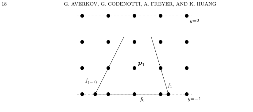
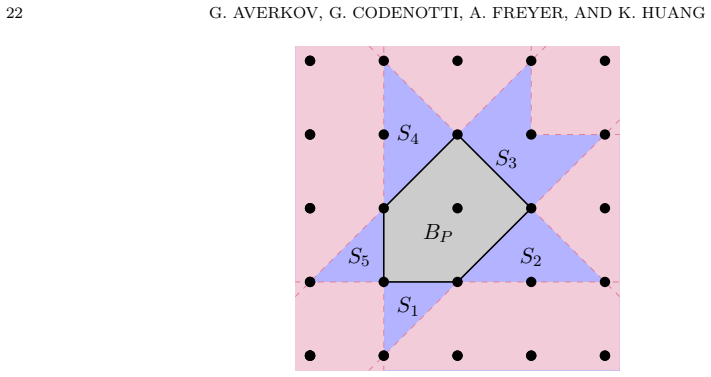
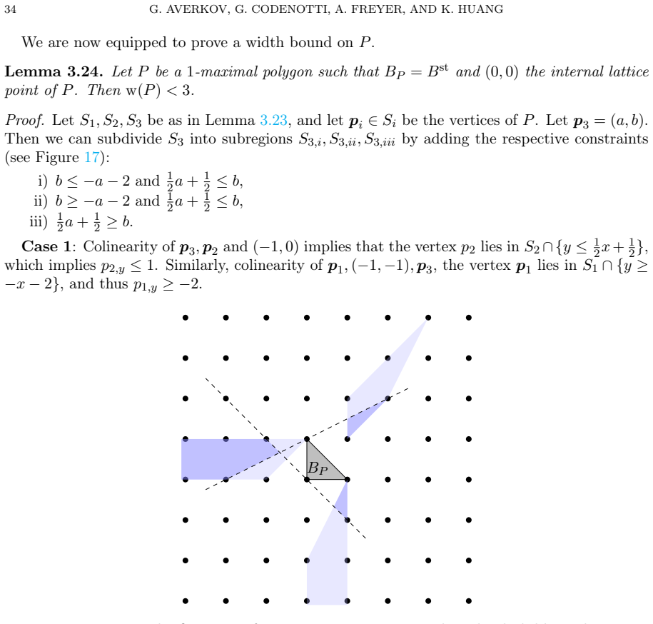
[Figure 1] Figure 1 (case-analysis diagram): The diagram illustrating the relative positions of the interior point is useful, but the arrows indicating the minimal-width direction and the lattice points should be labeled more clearly to match the textual cases.

Simulated Author's Rebuttal

0 responses · 0 unresolved

We thank the referee for their careful reading, positive evaluation, and recommendation of minor revision. The report accurately summarizes the main result establishing Flt(2,1)=3 and its applications. No specific major comments were raised in the report.

Circularity Check

0 steps flagged

No significant circularity identified

full rationale

The manuscript proves the central claim Flt(2,1)=3 via an exhaustive case analysis of the possible positions of the (at most one) interior lattice point relative to a minimal-width direction, together with an explicit convex body attaining width exactly 3. This argument rests only on the standard definitions of lattice width, supporting hyperplanes, and convex bodies in the plane with respect to Z^2; no quantity is fitted to data and then renamed as a prediction, no self-citation supplies a load-bearing uniqueness theorem or ansatz, and the equality is not obtained by construction from the inputs. Prior conjectures are cited only for context and do not enter the derivation chain.

Axiom & Free-Parameter Ledger

0 free parameters · 3 axioms · 0 invented entities

The work rests on standard axioms of convex geometry and the integer lattice; no free parameters, new entities, or ad-hoc assumptions are introduced in the abstract.

axioms (3)

standard math Convex bodies are closed subsets of R^d that contain the line segment between any two of their points.
Used in the definition of interior lattice points and lattice width.
standard math The lattice is the standard integer lattice Z^d with the usual Euclidean norm for width calculations.
Basis for the flatness constant Flt(d,k) and all lattice-point counting.
domain assumption Lattice width is defined via the minimum over integer directions of the difference between supporting hyperplanes.
Central to the statement that width is at most 3.

pith-pipeline@v0.9.0 · 5430 in / 1373 out tokens · 77423 ms · 2026-05-07T10:24:11.516300+00:00 · methodology

discussion (0)

Reference graph

Works this paper leans on

56 extracted references · 2 canonical work pages

[1]

Alexander, M

M. Alexander, M. Henk, and A. Zvavitch. A discrete version of Koldobsky’s slicing inequality.Israel J. Math., 222(1):261–278, 2017

2017
[2]

A. Aliev. The exact bound for the reverse isodiametric problem in 3-space.Rev. R. Acad. Cienc. Exactas Fís. Nat. Ser. A Mat. RACSAM, 118(3):Paper No. 111, 22, 2024

2024
[3]

Alonso-Gutiérrez, E

D. Alonso-Gutiérrez, E. Lucas, and J. Yepes Nicolás. On Rogers-Shephard-type inequalities for the lattice point enumerator.Commun. Contemp. Math., 25(8):Paper No. 2250022, 30, 2023

2023
[4]

Ambro and A

F. Ambro and A. Ito. Successive minima of line bundles.Adv. Math., 365:107045, 38, 2020. EXACT FLATNESS CONSTANT 43

2020
[5]

G. Averkov. A proof of Lovász’s theorem on maximal lattice-free sets.Beitr. Algebra Geom., 54(1):105–109, 2013

2013
[6]

Averkov, A

G. Averkov, A. Basu, and J. Paat. Approximation of corner polyhedra with families of intersection cuts. SIAM Journal on Optimization, 28(1):904–929, 2018

2018
[7]

Averkov, G

G. Averkov, G. Codenotti, A. Macchia, and F. Santos. A local maximizer for lattice width of 3-dimensional hollow bodies.Discrete Applied Mathematics, 298:129–142, 2021

2021
[8]

Averkov, M

G. Averkov, M. Conforti, A. Del Pia, M. Di Summa, and Y. Faenza. On the convergence of the affine hull of the chvátal–gomory closures.SIAM Journal on Discrete Mathematics, 27(3):1492–1502, 2013

2013
[9]

Averkov, B

G. Averkov, B. González Merino, I. Paschke, M. Schymura, and S. Weltge. Tight bounds on discrete quan- titative Helly numbers.Adv. Math., 89:76–101, 2017

2017
[10]

Averkov, J

G. Averkov, J. Hofscheier, and B. Nill. Generalized flatness constants, spanning lattice polytopes, and the Gromov width.Manuscripta Math., 170(1-2):147–165, 2023

2023
[11]

Averkov, J

G. Averkov, J. Krümpelmann, and S. Weltge. Notions of maximality for integral lattice-free polyhedra: the case of dimension three.Mathematics of Operations Research, 42(4):1035–1062, 2017

2017
[12]

Averkov, C

G. Averkov, C. Wagner, and R. Weismantel. Maximal lattice-free polyhedra: finiteness and an explicit description in dimension three.Mathematics of Operations Research, 36(4):721–742, 2011

2011
[13]

E. Balas. Integer programming and convex analysis: Intersection cuts from outer polars.Mathematical Programming, 2(1):330–382, 1972

1972
[14]

Balas.Disjunctive programming

E. Balas.Disjunctive programming. Springer, 2018

2018
[16]

Banaszczyk

W. Banaszczyk. Inequalities for convex bodies and polar reciprocal lattices inRn.Discrete Comput. Geom., 13(2):217–231, 1995

1995
[17]

Banaszczyk

W. Banaszczyk. Inequalities for convex bodies and polar reciprocal lattices inRn. II. Application ofK- convexity.Discrete Comput. Geom., 16(3):305–311, 1996

1996
[18]

Banaszczyk, A

W. Banaszczyk, A. E. Litvak, A. Pajor, and J. Stanislaw. The flatness theorem for nonsymmetric convex bodies via the local symmetry of Banach spaces.Math. Oper. Res., 24(3):728–750, 1999

1999
[19]

Bárány and Z

I. Bárány and Z. Füredi. On the lattice diameter of a convex polygon.Discrete Math., 241(1-3):41–50, 2001

2001
[20]

Bochnak, M

J. Bochnak, M. Coste, and M.-F. Roy.Real algebraic geometry, volume 36. Springer Science & Business Media, 2013

2013
[21]

Bohnert and J

M. Bohnert and J. Springer. Classifying rational polygons with small denominator and few interior lattice points.arXiv preprint arXiv:2410.17244, 2024

work page arXiv 2024
[22]

Codenotti and A

G. Codenotti and A. Freyer. Lattice reduced and complete convex bodies.J. Lond. Math. Soc. (2), 110(4):Pa- per No. e12982, 39, 2024

2024
[23]

Codenotti, T

G. Codenotti, T. Hall, and J. Hofscheier. Generalised flatness constants: A framework applied in dimension
[24]

Preprint arXiv:2110.02770, 2021

work page arXiv 2021
[25]

Codenotti and F

G. Codenotti and F. Santos. Hollow polytopes of large width.Proc. Am. Math. Soc., 148:1, 06 2019

2019
[26]

Conforti, G

M. Conforti, G. Cornuéjols, and G. Zambelli. Integer programming models. InInteger Programming, pages 45–84. Springer, 2014

2014
[27]

D. A. Cox, J. B. Little, and D. O’Shea. Ideals, varieties, and algorithms.American Mathematical Monthly, 101:656, 2025

2025
[28]

Dadush.Integer programming, lattice algorithms, and deterministic volume Estimation

D. Dadush.Integer programming, lattice algorithms, and deterministic volume Estimation. Georgia Institute of Technology, USA, 2012

2012
[29]

S. Dash, N. B. Dobbs, O. Günlük, T. J. Nowicki, and G. M. Świrszcz. Lattice-free sets, multi-branch split disjunctions, and mixed-integer programming.Mathematical Programming, 145(1):483–508, 2014

2014
[30]

Fejes Tóth and E

L. Fejes Tóth and E. Makai, Jr. On the thinnest non-separable lattice of convex plates.Studia Sci. Math. Hungar., 9:191–193, 1974

1974
[31]

Freyer and M

A. Freyer and M. Henk. Bounds on the lattice point enumerator via slices and projections.Discrete Comput. Geom., 67:895–918, 2022

2022
[32]

Freyer and M

A. Freyer and M. Henk. Polynomial bounds in Koldobsky’s discrete slicing problem.Proc. Amer. Math. Soc., 152(7):3063–3074, 2024

2024
[33]

Freyer and E

A. Freyer and E. Lucas. Interpolating between volume and lattice point enumerator with successive minima. Monatsh. Math., 198:717–740, 2022

2022
[34]

Gardner, P

R. Gardner, P. Gronchi, and C. Zong. Sums, projections, and sections of lattice sets, and the discrete covariogram.Discrete Comput. Geom., 34(2):391–409, 2005

2005
[35]

R. J. Gardner and P. Gronchi. A Brunn-Minkowski inequality for the integer lattice.Trans. Amer. Math. Soc., 353(10):3995–4024, 2001

2001
[36]

Griva, S

I. Griva, S. G. Nash, and A. Sofer.Linear and Nonlinear Optimization 2nd Edition. Society for Industrial and Applied Mathematics, Philadelphia, PA, 2008. 44 G. A VERKOV, G. CODENOTTI, A. FREYER, AND K. HUANG

2008
[37]

P. M. Gruber and C. G. Lekkerkerker.Geometry of Numbers. North-Holland, second edition, 1987

1987
[38]

Haase and J

C. Haase and J. Schicho. Lattice polygons and the number 2i + 7.The American Mathematical Monthly, 116(2):151–165, 2009

2009
[39]

Halikias, B

D. Halikias, B. Klartag, and B. A. Slomka. Discrete variants of Brunn-Minkowski type inequalities.Ann. Fac. Sci. Toulouse Math. (6), 30(2):267–279, 2021

2021
[40]

D.Hättig, J.Hausen, andJ.Springer.Classifyinglogdelpezzosurfaceswithtorusaction.Revista Matemática Complutense, pages 1–74, 2025

2025
[41]

Henk and F

M. Henk and F. Xue. On successive minima-type inequalities for the polar of a convex body.Rev. R. Acad. Cienc. Exactas Fís. Nat. Ser. A Mat. RACSAM, 113(3):2601–2616, 2019

2019
[42]

Old and recent problems for a new generation

A. G. Horváth. On convex bodies that are characterizable by volume function. “Old and recent problems for a new generation”: a survey.Arnold Math. J., 6(1):1–20, 2020

2020
[43]

C. A. J. Hurkens. Blowing up convex sets in the plane.Linear Algebra Appl., 134:121–128, 1990

1990
[44]

Iglesias, J

D. Iglesias, J. Yepes Nicolás, and A. Zvavitch. Brunn-Minkowski type inequalities for the lattice point enumerator.Adv. Math., 370:107193, 25, 2020

2020
[45]

Iglesias-Valiño and F

Ó. Iglesias-Valiño and F. Santos. Classification of empty lattice 4-simplices of width larger than 2.Trans. Amer. Math. Soc., 371:6605–6625, 2019

2019
[46]

R.KannanandL.Lovasz.Coveringminimaandlattice-point-freeconvexbodies.Ann. Math. (2), 128(3):577– 602, 1988

1988
[47]

H. W. Lenstra. Integer programming with a fixed number of variables.Math. Oper. Res., 8(4):538–548, 1983

1983
[48]

Lovász.Geometry of numbers and integer programming, pages 177–201

L. Lovász.Geometry of numbers and integer programming, pages 177–201. Kluwer Academic Publishers, 1989

1989
[49]

Makai, Jr

E. Makai, Jr. On the thinnest nonseparable lattice of convex bodies.Studia Sci. Math. Hungar., 13(1-2):19– 27, 1978

1978
[50]

Mayrhofer, J

L. Mayrhofer, J. Schade, and S. Weltge. Lattice-free simplices with lattice width2d−o(d). InInteger Programming and Combinatorial Optimization: 23rd International Conference, IPCO 2022, Eindhoven, The Netherlands, June 27–29, 2022, Proceedings, page 375–386, Berlin, Heidelberg, 2022. Springer-Verlag

2022
[51]

S. Mori, D. R. Morrison, and I. Morrison. On four-dimensional terminal quotient singularities.Mathematics of computation, 51(184):769–786, 1988

1988
[52]

J. Pál. Ein Minimierungsproblem für Ovale.Math. Ann., 83:311–319, 1921

1921
[53]

Rabinowitz

S. Rabinowitz. A census of convex lattice polygons with at most one interior lattice point.Ars Combinatoria, 28, 01 1989

1989
[54]

Reis and T

V. Reis and T. Rothvoss. The subspace flatness conjecture and faster integer programming. In2023 IEEE 64th Annual Symposium on Foundations of Computer Science—FOCS 2023, pages 974–988. IEEE Computer Soc., Los Alamitos, CA, [2023]©2023

2023
[55]

Scheiderer.A course in real algebraic geometry

C. Scheiderer.A course in real algebraic geometry. Springer, 2024

2024
[56]

Schneider.Convex bodies: The Brunn-Minkowski Theory

R. Schneider.Convex bodies: The Brunn-Minkowski Theory. Cambridge University press, second expanded edition, 2014

2014
[57]

https://www.sagemath.org

The Sage Developers.SageMath, the Sage Mathematics Software System (Version 9.4), 2022. https://www.sagemath.org. FU Berlin, AG Diskrete Geometrie und Topologische Kombinatorik, Arnimallee 2, 14195 Berlin, Germany Email address:{giulia.codenotti, a.freyer}@fu-berlin.de Brandenburg University of Technology Cottbus-Senftenberg, Platz der Deutschen Einheit 1...

2022