When Do Diffusion Models learn to Generate Multiple Objects?
Pith reviewed 2026-07-01 08:04 UTC · model grok-4.3
The pith
Diffusion models fail at multi-object scenes mainly because of scene complexity and held-out combinations, not concept imbalance.
A machine-rendered reading of the paper's core claim, the machinery that carries it, and where it could break.
Core claim
Training diffusion models on mosaic datasets, which vary the number of objects, concept balance, and held-out combinations, shows that scene complexity exerts the strongest influence on generation failures, counting accuracy is uniquely sensitive to low data volume, and compositional generalization degrades as the fraction of withheld concept combinations increases.
What carries the argument
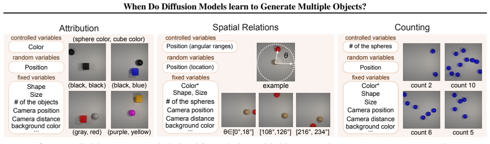
The mosaic framework, a controlled synthetic data generator that separately varies multi-object spatial relations, attribute assignments, and object counts while holding concept frequencies and combination coverage fixed.
If this is right
- Scene complexity affects multi-object generation success more strongly than uneven concept frequencies.
- Counting performance degrades more than other tasks when training data is scarce.
- Compositional generalization to new concept pairs collapses once the number of withheld combinations grows.
- The identified failure patterns appear consistently across the tested range of dataset sizes.
Where Pith is reading between the lines
- Real-world image collections may contain similar hidden compositional gaps even when overall concept counts look balanced.
- Architectures that add explicit mechanisms for tracking object counts or relations could bypass some of the observed limits.
- Data curation that deliberately increases exposure to high-complexity scenes might yield larger gains than further balancing of single-concept frequencies.
Load-bearing premise
The synthetic scenes created by the mosaic framework produce the same kinds of failures that appear in real training data without adding new artifacts from the data-generation process itself.
What would settle it
Train identical diffusion models on a real photograph dataset whose concept frequencies and pairwise combinations have been matched to the mosaic controls and check whether the same ranking of failure modes by scene complexity and counting holds.
Figures


read the original abstract
Text-to-image diffusion models achieve impressive visual fidelity, yet they remain unreliable in multi-object generation. Despite extensive empirical evidence of these failures, the underlying causes remain unclear. We begin by asking how much of this limitation arises from the data itself. To disentangle data effects, we consider two regimes across different dataset sizes: (1) concept generalization, where each individual concept is observed during training under potentially imbalanced data distributions, and (2) compositional generalization, where specific combinations of concepts are systematically held out. To study these regimes, we introduce mosaic (Multi-Object Spatial relations, AttrIbution, Counting), a controlled framework for dataset generation. By training diffusion models on mosaic, we find that scene complexity plays a dominant role rather than concept imbalance, and that counting is uniquely difficult to learn in low-data regimes. Moreover, compositional generalization collapses as more concept combinations are held out during training. These findings highlight fundamental limitations of diffusion models and motivate stronger inductive biases and data design for robust multi-object compositional generation.
Editorial analysis
A structured set of objections, weighed in public.
Referee Report
Summary. The paper claims that text-to-image diffusion models' failures in multi-object generation are driven primarily by scene complexity rather than concept imbalance. Using a new controlled 'mosaic' dataset generator, it studies concept generalization (under imbalance) versus compositional generalization (with held-out combinations) across dataset sizes, concluding that object count dominates, counting is uniquely hard in low-data regimes, and compositional performance collapses as more combinations are withheld.
Significance. If the claimed disentanglement holds, the work supplies useful empirical guidance on data effects in diffusion models for multi-object scenes and introduces a reusable controlled generator (mosaic) that could support further studies. The emphasis on counting and compositional hold-outs identifies concrete failure modes worth targeting with stronger inductive biases or data design.
major comments (1)
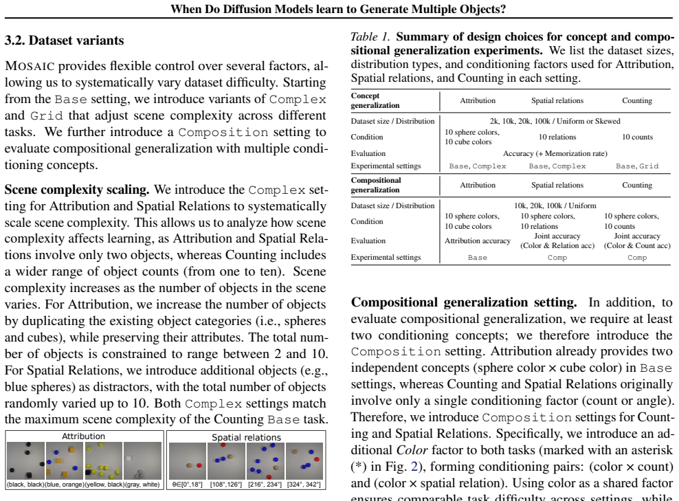
- [Mosaic framework] Mosaic framework (dataset generation procedure): increasing object count necessarily expands the space of possible attribute/relation tuples via combinatorial growth. The manuscript does not describe an explicit control that holds the number of distinct combinations fixed across complexity levels (e.g., via post-hoc matching or constrained sampling). Without this, the performance drop attributed to scene complexity could instead reflect reduced effective coverage of combinations, undermining the central claim that complexity dominates imbalance.
Simulated Author's Rebuttal
We thank the referee for their constructive feedback on our manuscript. We address the major comment below.
read point-by-point responses
-
Referee: [Mosaic framework] Mosaic framework (dataset generation procedure): increasing object count necessarily expands the space of possible attribute/relation tuples via combinatorial growth. The manuscript does not describe an explicit control that holds the number of distinct combinations fixed across complexity levels (e.g., via post-hoc matching or constrained sampling). Without this, the performance drop attributed to scene complexity could instead reflect reduced effective coverage of combinations, undermining the central claim that complexity dominates imbalance.
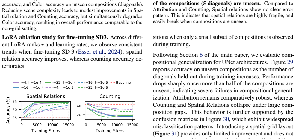
Authors: The referee correctly identifies a potential confound. The Mosaic framework fixes the underlying vocabulary of object types, attributes, and relations, but we did not enforce an identical number of distinct tuples across object-count levels. We will revise the manuscript to (1) explicitly report the number of unique combinations observed at each complexity level and (2) add controlled experiments that subsample training data to hold the number of observed combinations fixed while varying object count. This will allow a cleaner test of whether scene complexity remains the dominant factor. revision: yes
Circularity Check
No circularity: purely empirical study with no derivation chain
full rationale
The paper is an empirical investigation that introduces a synthetic dataset generator (mosaic) and reports observations from training diffusion models under controlled regimes of concept imbalance and compositional hold-outs. No equations, fitted parameters, predictions, uniqueness theorems, or ansatzes are present in the provided text or abstract. Central claims rest on experimental results rather than any reduction to inputs by construction. Self-citations, if present, are not load-bearing for any derivation. This matches the default expectation for non-circular empirical work.
Axiom & Free-Parameter Ledger
axioms (1)
- domain assumption The mosaic framework allows clean separation of concept generalization and compositional generalization regimes.
Reference graph
Works this paper leans on
-
[1]
Bonnaire, T., Urfin, R., Biroli, G., and M ´ezard, M. Why diffusion models don’t memorize: The role of implicit dynamical regularization in training.arXiv preprint arXiv:2505.17638,
-
[2]
Boo, H., Kim, H., Lee, M., Lee, S., Lee, J., Choi, J.-H., and Cho, H. Countsteer: Steering attention for object counting in diffusion models.arXiv preprint arXiv:2511.11253,
-
[3]
Bradley, A. Local mechanisms of compositional gen- eralization in conditional diffusion.arXiv preprint arXiv:2509.16447,
-
[4]
PixArt-$\alpha$: Fast Training of Diffusion Transformer for Photorealistic Text-to-Image Synthesis
Chen, J., Yu, J., Ge, C., Yao, L., Xie, E., Wu, Y ., Wang, Z., Kwok, J., Luo, P., Lu, H., et al. Pixart-alpha: Fast training of diffusion transformer for photorealistic text-to-image synthesis.arXiv preprint arXiv:2310.00426,
work page internal anchor Pith review Pith/arXiv arXiv
- [5]
-
[6]
Elmaaroufi, K., Lai, L., Svegliato, J., Bai, Y ., Seshia, S. A., and Zaharia, M. Graid: Enhancing spatial reasoning of vlms through high-fidelity data generation.arXiv preprint arXiv:2510.22118,
-
[7]
Farid, K., Sahay, R., Alnaggar, Y . A., Schrodi, S., Fischer, V ., Schmid, C., and Brox, T. What drives compositional gen- eralization in visual generative models?arXiv preprint arXiv:2510.03075,
work page internal anchor Pith review Pith/arXiv arXiv
-
[8]
Early-stopping too late? traces of memorization be- fore overfitting in generative diffusion
Garnier-Brun, J., Biggio, L., Mezard, M., and Saglietti, L. Early-stopping too late? traces of memorization be- fore overfitting in generative diffusion. InThe Impact of Memorization on Trustworthy Foundation Models: ICML 2025 Workshop,
2025
-
[9]
LoRA: Low-Rank Adaptation of Large Language Models
Hu, E. J., Shen, Y ., Wallis, P., Allen-Zhu, Z., Li, Y ., Wang, S., Wang, L., and Chen, W. Lora: Low-rank adaptation of large language models. arxiv 2021.arXiv preprint arXiv:2106.09685, 10,
work page internal anchor Pith review Pith/arXiv arXiv 2021
-
[10]
Jeong & Uselis, Y ., Uselis, A., Oh, S. J., and Rohrbach, A. Diffusion classifiers understand compositionality, but conditions apply.arXiv preprint arXiv:2505.17955, 2,
-
[11]
A new approach to linear filtering and prediction problems
Kamb, M. and Ganguli, S. An analytic theory of creativ- ity in convolutional diffusion models.arXiv preprint arXiv:2412.20292,
-
[12]
How Far is Video Generation from World Model: A Physical Law Perspective
Kang, B., Yue, Y ., Lu, R., Lin, Z., Zhao, Y ., Wang, K., Huang, G., and Feng, J. How far is video generation from world model: A physical law perspective.arXiv preprint arXiv:2411.02385,
work page internal anchor Pith review Pith/arXiv arXiv
-
[13]
Kang, S., Han, W., Ju, D., and Hwang, S. J. Rare text semantics were always there in your diffusion transformer. arXiv preprint arXiv:2510.03886, 2025a. Kang, W., Galim, K., Koo, H. I., and Cho, N. I. Counting guidance for high fidelity text-to-image synthesis. In 2025 IEEE/CVF Winter Conference on Applications of Computer Vision (WACV), pp. 899–908. IEEE...
-
[14]
Kingma, D. P. and Welling, M. Auto-encoding variational bayes.arXiv preprint arXiv:1312.6114,
work page internal anchor Pith review Pith/arXiv arXiv
-
[15]
Decoupled Weight Decay Regularization
Loshchilov, I. and Hutter, F. Decoupled weight decay regu- larization.arXiv preprint arXiv:1711.05101,
work page internal anchor Pith review Pith/arXiv arXiv
-
[16]
Oord, A. v. d., Li, Y ., and Vinyals, O. Representation learn- ing with contrastive predictive coding.arXiv preprint arXiv:1807.03748,
work page internal anchor Pith review Pith/arXiv arXiv
-
[17]
An Introduction to Convolutional Neural Networks
O’shea, K. and Nash, R. An introduction to convolutional neural networks.arXiv preprint arXiv:1511.08458,
work page internal anchor Pith review Pith/arXiv arXiv
-
[18]
Zaki, Luca Ambrogioni, and Dmitry Krotov
Pham, B., Raya, G., Negri, M., Zaki, M. J., Ambrogioni, L., and Krotov, D. Memorization to generalization: Emergence of diffusion models from associative memory. arXiv preprint arXiv:2505.21777,
-
[19]
SDXL: Improving Latent Diffusion Models for High-Resolution Image Synthesis
Podell, D., English, Z., Lacey, K., Blattmann, A., Dockhorn, T., M ¨uller, J., Penna, J., and Rombach, R. Sdxl: Im- proving latent diffusion models for high-resolution image synthesis.arXiv preprint arXiv:2307.01952,
work page internal anchor Pith review Pith/arXiv arXiv
-
[20]
Ramesh, A., Dhariwal, P., Nichol, A., Chu, C., and Chen, M
URL https: //arxiv.org/abs/2507.10768. Ramesh, A., Dhariwal, P., Nichol, A., Chu, C., and Chen, M. Hierarchical text-conditional image generation with clip latents.arXiv preprint arXiv:2204.06125, 1(2):3,
-
[21]
U-net: Con- volutional networks for biomedical image segmenta- tion
Ronneberger, O., Fischer, P., and Brox, T. U-net: Con- volutional networks for biomedical image segmenta- tion. InMedical image computing and computer-assisted intervention–MICCAI 2015: 18th international confer- ence, Munich, Germany, October 5-9, 2015, proceedings, part III 18, pp. 234–241,
2015
-
[22]
Score-Based Generative Modeling through Stochastic Differential Equations
Song, Y ., Sohl-Dickstein, J., Kingma, D. P., Kumar, A., Er- mon, S., and Poole, B. Score-based generative modeling through stochastic differential equations.arXiv preprint arXiv:2011.13456,
work page internal anchor Pith review Pith/arXiv arXiv 2011
-
[23]
URL https: //arxiv.org/abs/2505.09388. Thrush, T., Jiang, R., Bartolo, M., Singh, A., Williams, A., Kiela, D., and Ross, C. Winoground: Probing vision and language models for visio-linguistic compositionality. In Proceedings of the IEEE/CVF Conference on Computer Vision and Pattern Recognition, pp. 5238–5248,
work page internal anchor Pith review Pith/arXiv arXiv
-
[24]
Toker, M., Orgad, H., Ventura, M., Arad, D., and Belinkov, Y . Diffusion lens: Interpreting text encoders in text-to- image pipelines.arXiv preprint arXiv:2403.05846,
- [25]
- [26]
-
[27]
Wiedemer, T., Sharma, Y ., Prabhu, A., Bethge, M., and Brendel, W. Pretraining frequency predicts compositional generalization of clip on real-world tasks.arXiv preprint arXiv:2502.18326,
-
[28]
Omnigen: Uni- fied image generation.arXiv preprint arXiv:2409.11340,
Xiao, S., Wang, Y ., Zhou, J., Yuan, H., Xing, X., Yan, R., Li, C., Wang, S., Huang, T., and Liu, Z. Omnigen: Uni- fied image generation.arXiv preprint arXiv:2409.11340,
-
[29]
1.58-bit flux.arXiv preprint arXiv:2412.18653, 2024a
Yang, C., Liu, C., Deng, X., Kim, D., Mei, X., Shen, X., and Chen, L.-C. 1.58-bit flux.arXiv preprint arXiv:2412.18653, 2024a. Yang, Y ., Park, C. F., Lubana, E. S., Okawa, M., Hu, W., and Tanaka, H. Swing-by dynamics in concept learn- ing and compositional generalization.arXiv preprint arXiv:2410.08309, 2024b. Yoo, N., Russakovsky, O., and Zhu, Y . D2d: ...
-
[30]
Mitigating compositional issues in text-to-image generative models via enhanced text embeddings
Zarei, A., Rezaei, K., Basu, S., Saberi, M., Moayeri, M., Kattakinda, P., and Feizi, S. Mitigating compositional issues in text-to-image generative models via enhanced text embeddings. Zhang, Z., Hu, F., Lee, J., Shi, F., Kordjamshidi, P., Chai, J., and Ma, Z. Do vision-language models represent space and how? evaluating spatial frame of reference under a...
-
[31]
1” or “one
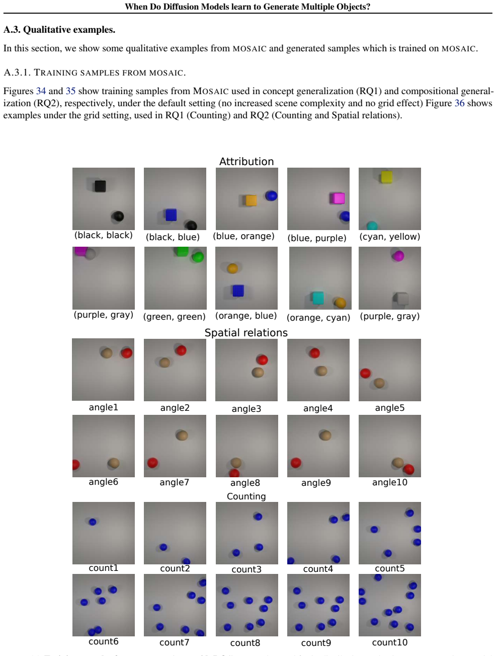
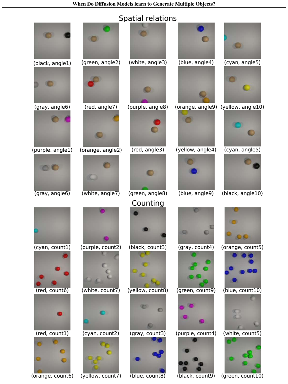
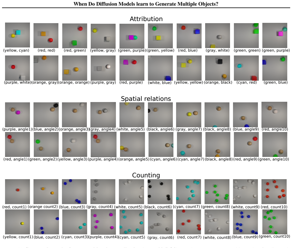
13 When Do Diffusion Models learn to Generate Multiple Objects? A. Appendix This supplemental material provides detailed experimental setup (Section A.1), extended experimental results (Sec- tion A.2), and qualitative examples (Section A.3). First, we describe experimental details, including those for Fig- ure 1 (b) in main paper, MOSAIC, design choices, ...
2022
-
[32]
Prompt:Find number words (one, two, three, four, five, six, seven, eight, nine, ten) that appear next to or very close to nouns describing countable physical things of any size
with carefully designed prompts. Prompt:Find number words (one, two, three, four, five, six, seven, eight, nine, ten) that appear next to or very close to nouns describing countable physical things of any size. ONLY count when: - The number word is adjacent to or within 1-2 words of a concrete noun (like: two dogs, one red car, three small boxes, four tal...
2019
-
[33]
Following their object list, we uniformly generate 830 prompts for each target count
on counting using prompts derived from CompBench (Huang et al., 2023). Following their object list, we uniformly generate 830 prompts for each target count. Evaluation follows the CompBench protocol, which uses UniDet (Zhou et al.,
2023
-
[34]
in front of
If none found, all counts should be 0 Figure 17 shows that some spatial relation terms appear far more frequently than others, indicating a substantial imbalance in the Laion2B caption. This confirms that our concept imbalance design is not only relevant for analyzing counting, but also extends more broadly to spatial relations. in front of above behind b...
2024
-
[35]
For example, in a 100k dataset, theskeweddistribution allocates (22,550, 17,950, 14,350, 11,450, 9,150, 7,300, 5,850, 4,650, 3,750, 3,000) samples across the ten classes
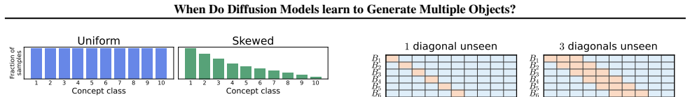
Class imbalance details.For theskewedsetting, we construct datasets with controlled degrees of class imbal- ance while keeping the skewness pattern consistent across different dataset sizes. For example, in a 100k dataset, theskeweddistribution allocates (22,550, 17,950, 14,350, 11,450, 9,150, 7,300, 5,850, 4,650, 3,750, 3,000) samples across the ten clas...
2025
-
[36]
for the optimizer. 15 When Do Diffusion Models learn to Generate Multiple Objects? Table 4.Compositional configuration for Count × Color (Count- ing).Diagonal indices specify the order in which concept pairs are removed to create unseen composition settings. Higher unseen- diagonal counts correspond to harder compositional generalization. RED GREEN BLUE Y...
-
[37]
We adopt the DiT architecture from SD3 (Esser et al.,
trained with rectified flow objectives (Lip- man et al., 2023). We adopt the DiT architecture from SD3 (Esser et al.,
2023
-
[38]
To ensure comparable image quality across architectures, we fix the V AE to the one used in SD2, which is also used for all UNet-based experiments in this work
and reduce the model size to approximately 90M parameters to closely match the capacity of our UNet-based baseline. To ensure comparable image quality across architectures, we fix the V AE to the one used in SD2, which is also used for all UNet-based experiments in this work. In the original SD3 design, text embeddings are injected through two pathways: (...
2024
-
[39]
17 When Do Diffusion Models learn to Generate Multiple Objects? 0.6 0.8 1.0Accuracy Uniform Skewed 2k 10k20k50k 100k Dataset Size 0.0 0.5 1.0Memorization Model Size 40M 90M (Ours) 200M 2k 10k20k50k 100k Dataset Size Model Size 40M 90M (Ours) 200M Figure 18.Influence of model size on Counting accuracy.Larger or smaller models do not mitigate the failure at...
2000
-
[40]
We also evaluate a frozen condition encoder (red) that is pretrained with cross-entropy loss and not jointly optimized with the diffusion model
(orange). We also evaluate a frozen condition encoder (red) that is pretrained with cross-entropy loss and not jointly optimized with the diffusion model. However, as shown in Figure 26 (bottom), the embedding collapse persists even with these objectives, indicating that the issue does not stem solely from inade- quate supervision of the condition encoder...
2024
-
[41]
provides only limited improvement and does not recover compositional generalization. Overall, the failure mode remains unchanged: increasing dataset scale alone is insufficient, and compositional generalization does not reli- ably emerge even with a stronger architecture and improved training objectives. Is a compositionally broken text encoder responsibl...
2024
-
[42]
26 When Do Diffusion Models learn to Generate Multiple Objects? A.3.2
8 9 106 7 (yellow, angle7) (purple, angle8) (white, angle9) (black, angle10)(green, angle6) Figure 36.Training samples fromMOSAICunder grid layout (RQ1 and RQ2).Explicit spatial priors simplify scene structure, leading to improved counting and relational stability but reduced texture variation. 26 When Do Diffusion Models learn to Generate Multiple Object...
2024
discussion (0)
Sign in with ORCID, Apple, or X to comment. Anyone can read and Pith papers without signing in.