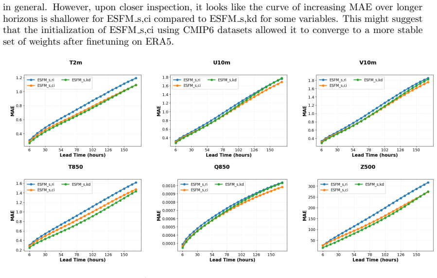
arxiv: 2605.00850 · v1 · submitted 2026-04-20 · ⚛️ physics.ao-ph · cs.AI· cs.LG· eess.IV

Recognition: unknown

Earth System Foundation Model (ESFM): A unified framework for heterogeneous data integration and forecasting

Benedikt Soja, Dana Grund, Fanny Lehmann, Firat Ozdemir, Leonardo Trentini, Mathieu Salzmann, Oliver Fuhrer, Salman Mohebi, Sebastian Schemm, Siddhartha Mishra, Simon Adamov, Torsten Hoefler, Yun Cheng, Zhenyi Zhang

Pith reviewed 2026-05-10 03:18 UTC · model grok-4.3

classification ⚛️ physics.ao-ph cs.AIcs.LGeess.IV

keywords Earth systemfoundation modelheterogeneous datamissing valuesaxial attentionvariable tokenizationweather forecastingclimate prediction

0 comments

The pith

ESFM predicts variables in unobserved regions by preserving inter-variable physical relationships.

A machine-rendered reading of the paper's core claim, the machinery that carries it, and where it could break.

The paper presents ESFM, a foundation model extending the 3D Swin UNet to unify heterogeneous Earth system data including gridded, satellite, and station observations with missing values. Axial attention captures dependencies between variables, and individual variable tokenization allows flexible shuffling during training. This setup enables skillful prediction of variables where no initial data exists, such as certain pressure levels, while maintaining relationships like those among temperature, pressure, and humidity. A sympathetic reader would care because real-world data is often incomplete, so one versatile model reduces the need for task-specific systems and supports broader climate applications. Results on ERA5, CMIP6, MODIS, and station data show competitive performance, with good handling of extreme events.

Core claim

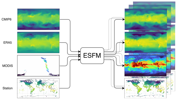
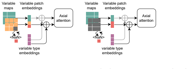
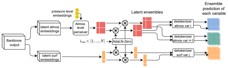
ESFM introduces axial attention to model inter-variable dependencies and per-variable tokenization to handle varying sets of inputs. Trained on dense gridded data like ERA5 and CMIP6 as well as sparse satellite and station data, the model predicts variables in regions or pressure levels lacking initial observations. It preserves physical relationships, for example between temperature, pressure, and humidity. Adaptive layer norm enables probabilistic ensembles, and case studies confirm accurate extreme weather predictions while retaining long-term stability.

What carries the argument

Axial attention for inter-variable dependencies together with individual variable tokenization on the 3D Swin UNet backbone.

If this is right

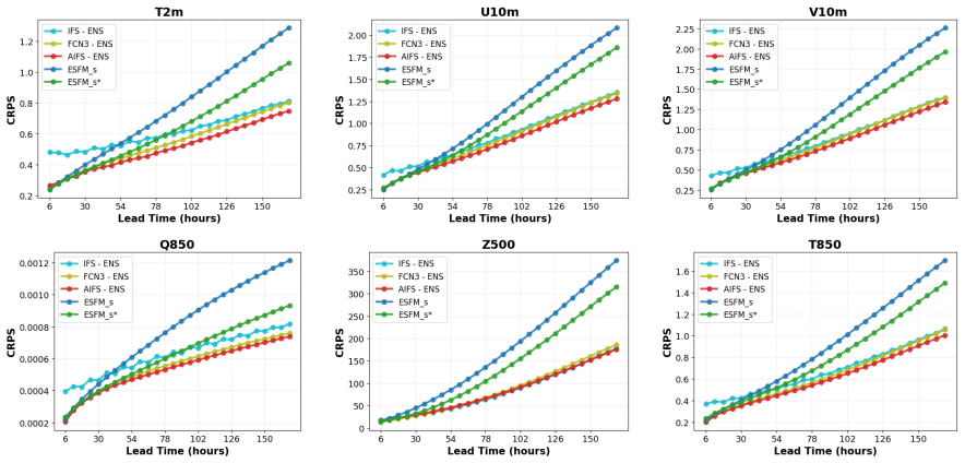
Competitive or superior performance on benchmarks using ERA5, CMIP6, regionally masked data, MODIS satellite data, and station data.
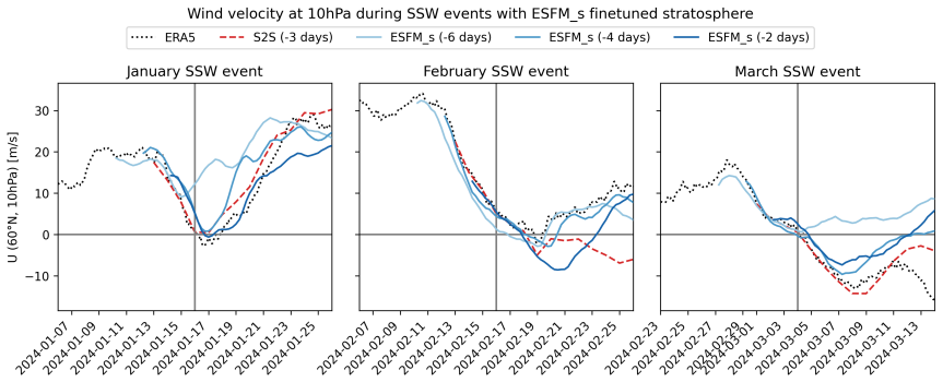
Accurate positional and magnitude estimates for extreme events such as Super Typhoon Doksuri and sudden stratospheric warming.
Simple transformation to probabilistic forecasting via adaptive layer norm ensembles.
Retention of long-term stability from previous foundation models.
Simplified building of extensions for new downstream tasks due to variable tokenization.

Where Pith is reading between the lines

These are editorial extensions of the paper, not claims the author makes directly.

Operational forecasting centers could adopt this as a base for multi-source data assimilation to improve predictions in data-poor areas.
Future work might verify whether the predictions satisfy fundamental conservation laws like mass or energy balance in the extrapolated regions.
The unified framework might lower barriers for researchers adding new variables or data types without retraining entire models.

Load-bearing premise

Axial attention and variable tokenization extensions allow generalization of physical relationships into unobserved regions without non-physical artifacts or conservation violations.

What would settle it

Independent validation showing that predicted temperature, pressure, and humidity fields in unobserved regions violate known physical correlations or conservation principles.

Figures

Figures reproduced from arXiv: 2605.00850 by Benedikt Soja, Dana Grund, Fanny Lehmann, Firat Ozdemir, Leonardo Trentini, Mathieu Salzmann, Oliver Fuhrer, Salman Mohebi, Sebastian Schemm, Siddhartha Mishra, Simon Adamov, Torsten Hoefler, Yun Cheng, Zhenyi Zhang.

**Figure 1.** Figure 1: ESFM unified framework: ESFM is a flexible foundation model, ingesting multi-modal heterogeneous datasets with missing, sparse, or point data, and predict forecasts with ensembles; all using the same backbone. 1 Introduction 1.1 Motivation Accurate weather forecasting is crucial for numerous applications in societal resilience, such as disaster mitigation and food security, and industrial sectors, includi… view at source ↗

**Figure 2.** Figure 2: ESFM encoder: ESFM tokenizes each input variable individually, then performs selfattention across variable tokens (i.e., axial attention). The size of the variable dimension is then reduced using a perceiver module for both atmospheric and surface variables. Observations across different pressure levels are tokenized separately and corresponding tokens across different pressure levels are aggregated to la… view at source ↗

**Figure 3.** Figure 3: ESFM training with missing data: Partial (left) or completely missing (right) input variable embeddings (shown in gray) are exchanged with a learnable NaN token (shown in red) in ESFM. ESFM introduces learnable NaN tokens, which replace input patches where part or all of the region within an input patch consists of missing observations. Internally, NaN tokens get positional encodings of the corresponding v… view at source ↗

**Figure 4.** Figure 4: ESFM training with station data: ECMWF 11k station data (left) is greedily mapped onto a compact irregular grid (middle & right). Stations are marked to indicate those that will be used for training (blue) and kept as holdout sets (red). 2.3 Deterministic to ensemble simulations Probabilistic prediction capability is crucial for most applications in the environmental sciences. We propose a simple means to … view at source ↗

**Figure 5.** Figure 5: ESFM decoder: The decoder structure of ESFM utilizes perceiver module to map latent atmospheric embeddings to queried set of target pressure levels, which does not have to be the same levels at observation. Using a set of queried ensemble members, latent ensembles are formed from latent embeddings using AdaLN-Zero layer, which are then passed through detokenizer of each variable to reconstruct variable pat… view at source ↗

**Figure 6.** Figure 6: Impact of pretraining on forecast performance: Six hour lead time forecast performance of ESFM s based on the different pretraining, shown in mean absolute error, and detailed in the schematic. Models are random initialization (ri), pretraining on 8 CMIP6 models (ci), and KD on pretrained Aurora (kd). First three rows show models trained with masking protocol. ESFM s,kd* in last row shows the performance … view at source ↗

**Figure 7.** Figure 7: Maximum wind velocity (left) and location (right) of Super Typhoon Doksuri 2023: (left) ERA5 (black), ESFM s (orange) and Aurora models initialized on 21.07.2023 at midnight: Aurora large (cyan dashed line), Aurora small (blue solid line), ESFM small with 8 probabilistic decoders. (right) Map of eastward wind velocity on 25.07.2023 (96- hour lead time). The IBTrACS best track is shown in all figures. 4.4 C… view at source ↗

**Figure 8.** Figure 8: Sudden stratospheric warming: Eastward wind velocity at 10 hPa and latitude 60◦N during three SSW events. Each panel shows one event, with the vertical line denoting the start of the SSW event. ESFM s is initialized on three dates up to 6 days before the SSW event (blue lines). The numerical S2S baseline model is initialized three days before the event (red dashed line). The wind velocity is averaged along… view at source ↗

**Figure 9.** Figure 9: Stratosphere-troposphere coupling: 500 hPa geopotential poleward of 30oN latitude averaged over the week following the January SSW, displayed as anomaly compared to the ERA5 climatology. Models are initialized two days before the event. (Left) ERA5 reference geopotential height anomaly, (middle) error in the anomaly predicted by the baseline ESFM, (right) error in the anomaly predicted by ESFM finetuned wi… view at source ↗

**Figure 10.** Figure 10: Multidecadal rollout stability The shown 25-year long rollout was initialized on 02.01.1959. The solid line shows the spatial average over Europe, and the shaded area shows the range from the spatial minimum to the spatial maximum. ERA5 is shown as a reference. Points are sampled every seven days. cycle and maintains physically realistic temperature distributions, as indicated by the shaded areas, closely… view at source ↗

**Figure 11.** Figure 11: Bounding boxes of the regions masked from the test set in experiments under Sec. 5.1.1. performance purely within the removed region for Switzerland, Europe, and the contiguous United States in [PITH_FULL_IMAGE:figures/full_fig_p017_11.png] view at source ↗

**Figure 12.** Figure 12: ), confirming that withholding an entire continent’s observations from the initial conditions 0.00000 0.00025 0.00050 0.00075 0.00100 0.00125 0.00150 | GH| [m/m] 0 10 20 30 40 50 60 70 W S [m / s] No Masking Prediction Target Geostrophic: Ug = (g/f)| GH| Wind speed = 0 Wind speed < 0 (unphysical) 0.00000 0.00025 0.00050 0.00075 0.00100 0.00125 0.00150 | GH| [m/m] Masking Europe 10 0 10 1 10 2 10 3 10 4 10… view at source ↗

**Figure 13.** Figure 13: Physical consistency: Joint density of U10m and V10m evaluated over Europe (35°N– 72°N, 25°W–50°E) for ESFM s under five distinct variable-masking configurations. In each panel a different variable is withhold from the initial conditions across all pressure and surface levels: U10m, V10m, U, V and Z. ESFM prediction (color); ERA5 reference (gray isolines). Note the logarithmic density scale. We further ex… view at source ↗

**Figure 14.** Figure 14: Physical consistency: Joint density of T and Q at 500 hPa evaluated over Europe (35°N–72°N, 25°W–50°E) for ESFM s without masking (left) and with the 500 hPa level withheld from the initial conditions (right). ERA5 reference (Gray isolines); ESFM prediction (color). Note the logarithmic density scale. The red dashed curve is qsat(T) following Bolton (1980). 20 [PITH_FULL_IMAGE:figures/full_fig_p020_14.png] view at source ↗

**Figure 15.** Figure 15: ESFM can handle very sparse observations for its prediction: Sample PWV observation (MOD05 IR) from MODIS at times t (input), t+1 (target), and forecasted PWV at time t+1 (six-hour lead time) by ESFM trained with masking protocol. 21 [PITH_FULL_IMAGE:figures/full_fig_p021_15.png] view at source ↗

**Figure 16.** Figure 16: ESFM forecast finetuned on MODIS satellite data: Comparison of six hour forecast of ESFM vs satellite observations (MOD05 IR based PWV) aggregated over Switzerland (left) and United Kingdom (right) for a sample week in 2024. 5.2.1 Fine tuning with sparse data To construct an hourly MODIS-based dataset, we aggregate swath observations collected within each 1-hour window (e.g., from HH:00 to HH:55) and as… view at source ↗

**Figure 17.** Figure 17: Stable rollout forecast initialized from sparse MODIS data: Two-week lead time forecast performance of MODIS IR and NIR based PWV variable throughout the test set of 2023–2024 measured in terms of mean absolute error (MAE, left) and Pearson correlation coefficient (PCC, right). Autoregressive rollouts are generated through 6 hour forecast steps. Despite the sparsity of the data, ESFM s is able to achieve … view at source ↗

**Figure 18.** Figure 18: shows validation set loss curves of ESFM s with four different initializations: (i) no pretraining, (ii) pretraining on eight CMIP6 datasets, (iii) pretraining on 8 CMIP6 datasets and ERA5, and (iv) pretraining on ERA5. Pretraining on CMIP6 datasets, whether alone or in addition to ERA5, yields a faster decrease of the loss function and stabilization to better accuracy than pretraining on ERA5 alone or wi… view at source ↗

**Figure 19.** Figure 19: RMSE on the test year 2023 when finetuning ESFM s with six new surface variables, starting from two pretrained models: baseline ESFM s (blue) and ESFM s pretrained with a subset Snew,1 of additional variables (orange). The plot shows variables from Snew,2 that are unseen for both pretrained models. The inner boxes show a zoom on lead times shorter than 24 hours. 6 Summary and discussion This study introd… view at source ↗

**Figure 20.** Figure 20: Schematic of the masking applied to the observations for masked ESFM [PITH_FULL_IMAGE:figures/full_fig_p036_20.png] view at source ↗

**Figure 21.** Figure 21: extends the geostrophic analysis of Sec. 5.1 to the thermodynamic dimension, showing the joint distribution of T and Q at 500 hPa evaluated within the withheld European domain. As in the pressure level masking case, the predicted distribution remains below the Bolton saturation curve and above zero in both configurations, confirming that the model does not generate thermodynamically inconsistent states wi… view at source ↗

**Figure 22.** Figure 22: As [PITH_FULL_IMAGE:figures/full_fig_p038_22.png] view at source ↗

**Figure 23.** Figure 23: Multi-tokenizer structure of ESFM. ESFM s with ensemble prediction, we use N=8 AdaLN based ensemble modulation parameters. For larger ensembles such as N=1000, we implemented a routine that randomly selects a subset of Ns=8 ensemble parameters to optimize for each training step. We use a combination of almost fair CRPS loss and MAE on the ensemble means with equal weight. A.3.1 Variable perceivers Token e… view at source ↗

**Figure 24.** Figure 24: Rollout forecasting MAE performance of ESFM s models depending on their pretraining objectives, up to seven days lead time, without any autoregressive finetuning. We also show autoregressive rollout based forecasting performance of ESFM s with respect to SotA models in [PITH_FULL_IMAGE:figures/full_fig_p040_24.png] view at source ↗

**Figure 25.** Figure 25: Rollout forecasting MAE performance of ESFM s trained without masking in comparison with SotA models up to seven days lead time [PITH_FULL_IMAGE:figures/full_fig_p041_25.png] view at source ↗

**Figure 26.** Figure 26: Rollout forecasting performance of ensemble ESFM s trained without masking in comparison with SotA models up to seven days lead time. For reference, we also include ESFM s*; autoregressively rollout finetuned ESFM s with a single LoRA layer for 3.4 k steps, up to 10 steps (60 hours lead time). Performance metric is MAE computed over the means of ensembles. 41 [PITH_FULL_IMAGE:figures/full_fig_p041_26.png] view at source ↗

**Figure 27.** Figure 27: Rollout forecasting CRPS performance of ensemble ESFM s trained without masking in comparison with SotA models up to seven days lead time. For reference, we also include ESFM s*; autoregressively rollout finetuned ESFM s with a single LoRA layer for 3.4 k steps, up to 10 steps (60 hours lead time). Appendix C. Datasets Here, we go over the contents of the datasets used in this work. C.1 ERA5 dataset Herei… view at source ↗

**Figure 28.** Figure 28: Training loss when finetuning ESFM s on a large set of new surface variables from two pretrained models: baseline pretraining (blue) and pretraining with a small set of new surface variables (orange). 47 [PITH_FULL_IMAGE:figures/full_fig_p047_28.png] view at source ↗

**Figure 29.** Figure 29: shows the maps of wind velocity in South-East Asia as the Doksuri typhoon progresses. Since the cyclone eye trajectory is extracted from the IBTrACS catalog and not computed from the models, it is placed at the same position across the compared models [PITH_FULL_IMAGE:figures/full_fig_p048_29.png] view at source ↗

read the original abstract

Foundation models (FMs) for the Earth system learn statistical relationships between physical variables across massive datasets to enable versatile downstream applications through finetuning, separating them from task-specific weather models. Here, we introduce Earth System Foundation Model (ESFM), a fully open model building on the 3D Swin UNet backbone of the pioneering Aurora model. ESFM introduces extensions that increase functionality and foster adoption in climate sciences. First, the encoding scheme and training protocols have been extended to handle diverse datasets, including those containing missing values across all spatio-temporal dimensions such as satellite data, as well as station data, all under one backbone. Axial attention is introduced to capture inter-variable dependencies. As a result ESFM skillfully predicts variables in regions or on pressure levels where no data is present at the initial time, while preserving inter-variable relationships, for example between temperature, pressure, and humidity. Individual variable tokenization enables different sets of variables to be shuffled during training and simplifies the process of building extensions for new downstream tasks. Adaptive layer norm-based ensembles allow for a simple yet effective way to transform deterministic ESFM to a probabilistic FM. We present findings using dense gridded data (ERA5, CMIP6), regionally masked dense data, sparse gridded MODIS satellite data, and station data. Results demonstrate competitive or superior performance relative to state-of-the-art benchmarks. Case studies of Super Typhoon Doksuri (2023) and 2024 sudden stratospheric warming events show accurate positional and magnitude estimations of extreme weather. ESFM retains the strengths of previous foundation models, such as long-term stability, but facilitates application to a variety of downstream tasks.

Editorial analysis

A structured set of objections, weighed in public.

Desk editor's note, referee report, simulated authors' rebuttal, and a circularity audit. Tearing a paper down is the easy half of reading it; the pith above is the substance, this is the friction.

Desk Editor's Note private letter to a colleague

ESFM extends Aurora practically for missing heterogeneous data but needs stronger quantitative and physical validation for its extrapolation claims.

read the letter

ESFM adds axial attention and variable-specific tokenization to Aurora to manage missing values across satellite and station data in a single model, but the support for its claims about physical relationship preservation in data voids is mostly qualitative. The work builds on the 3D Swin UNet from Aurora and extends the encoding and training to deal with diverse inputs that have gaps in space and time. This includes dense gridded reanalysis and climate model output, regionally masked data, sparse MODIS satellite observations, and station measurements. Axial attention is meant to capture dependencies between variables, while individual tokenization allows shuffling variable sets and easier addition of new tasks. Adaptive layer norm ensembles provide a way to generate probabilistic forecasts from the base deterministic model. These changes let the model attempt predictions on pressure levels or regions with no data at initialization, and the authors report that inter-variable links, such as temperature with pressure and humidity, are maintained. The case studies on the 2023 Super Typhoon Doksuri and the 2024 sudden stratospheric warming demonstrate reasonable accuracy in tracking extremes. The model also keeps the long-term stability seen in prior foundation models. On the evidence side, the abstract states competitive or superior results relative to benchmarks, but supplies no concrete metrics, ablation studies, or verification steps for the missing-data handling or the physical fidelity of the extrapolations. The training is purely data-driven, so there is no built-in mechanism to enforce conservation principles or thermodynamic consistency in the predicted fields for unobserved areas. That leaves the generalization claim as an assumption supported by the case studies rather than by targeted diagnostics. Researchers focused on machine learning applications to the Earth system will find this relevant, especially if they need a backbone that accommodates incomplete observations without separate models for each data type. The open release and the modular design for extensions could make it a practical starting point for downstream work in forecasting or risk assessment. The paper is coherent enough on its own terms to merit peer review. The architecture choices are described at a level that allows evaluation, and the empirical scope covers several data regimes. I would recommend sending it out for review, though the authors should expect questions about quantitative benchmarks and checks on physical plausibility in the masked regions.

Referee Report

3 major / 2 minor

Summary. The paper introduces the Earth System Foundation Model (ESFM), an extension of the 3D Swin UNet backbone from the Aurora model. It incorporates axial attention for inter-variable dependencies, individual variable tokenization to handle shuffled variable sets, and training protocols for heterogeneous data including missing values from satellite and station observations. The central claims are that ESFM can predict variables in fully unobserved spatial or pressure-level regions while preserving inter-variable physical relationships (e.g., temperature-pressure-humidity), achieves competitive or superior performance on ERA5, CMIP6, regionally masked, MODIS, and station data, and supports probabilistic ensembles via adaptive layer norm; case studies on Typhoon Doksuri and 2024 sudden stratospheric warming are presented as evidence of accurate extreme-event forecasting.

Significance. If the generalization claims hold with rigorous verification, ESFM would represent a meaningful advance in open foundation models for the Earth system by unifying dense, sparse, and missing-data sources under a single backbone and enabling downstream tasks without task-specific retraining. The open release and support for probabilistic outputs are additional strengths that could facilitate broader adoption in climate applications.

major comments (3)

[Abstract] Abstract and case-study sections: The headline claim that axial attention plus variable tokenization enables skillful prediction of variables (e.g., temperature, pressure, humidity) in regions or pressure levels with no initial data, while preserving inter-variable relationships, is supported only by qualitative case studies (Doksuri, SSW) and aggregate benchmark scores. No quantitative diagnostics—such as hydrostatic residual, moist-static-energy conservation, or thermodynamic consistency metrics—are reported specifically inside the masked or unobserved regions.
[Results] Results and methods sections: The manuscript states that results demonstrate competitive or superior performance on dense gridded, regionally masked, sparse MODIS, and station data, yet provides no ablation studies isolating the contribution of axial attention or per-variable tokenization to extrapolation into unobserved regions or to inter-variable preservation.
[Methods] Training protocols: The description indicates a purely statistical training objective with extensions for missing values across spatio-temporal dimensions, but supplies no details on how missing-data masking is implemented or whether any mechanism (loss term or architectural constraint) encourages physical consistency in the generated fields.

minor comments (2)

[Abstract] The abstract refers to 'adaptive layer norm-based ensembles' for probabilistic output but does not specify the implementation details or how ensemble spread is calibrated.
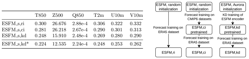
Quantitative performance numbers (RMSE, ACC, etc.) for the benchmark comparisons are absent from the abstract and high-level results summary, making the 'competitive or superior' statement difficult to evaluate without consulting tables or figures.

Simulated Author's Rebuttal

3 responses · 0 unresolved

We thank the referee for their constructive comments and positive assessment of the potential significance of ESFM. We address each of the major comments below and outline the revisions we will make to strengthen the manuscript.

read point-by-point responses

Referee: [Abstract] Abstract and case-study sections: The headline claim that axial attention plus variable tokenization enables skillful prediction of variables (e.g., temperature, pressure, humidity) in regions or pressure levels with no initial data, while preserving inter-variable relationships, is supported only by qualitative case studies (Doksuri, SSW) and aggregate benchmark scores. No quantitative diagnostics—such as hydrostatic residual, moist-static-energy conservation, or thermodynamic consistency metrics—are reported specifically inside the masked or unobserved regions.

Authors: We agree that additional quantitative evidence would strengthen the claims regarding the preservation of physical relationships in unobserved regions. In the revised manuscript, we will add quantitative diagnostics, including hydrostatic residual and thermodynamic consistency metrics, computed specifically within the masked and unobserved regions for the case studies and benchmarks. These will be included in the Results section to provide more rigorous support for the headline claims. revision: yes
Referee: [Results] Results and methods sections: The manuscript states that results demonstrate competitive or superior performance on dense gridded, regionally masked, sparse MODIS, and station data, yet provides no ablation studies isolating the contribution of axial attention or per-variable tokenization to extrapolation into unobserved regions or to inter-variable preservation.

Authors: We acknowledge the value of ablation studies for isolating the effects of axial attention and individual variable tokenization. We will perform and include additional ablation experiments in the revised manuscript. These will compare the full ESFM against variants without axial attention and without per-variable tokenization, evaluating their impact on performance in regionally masked and unobserved data scenarios, as well as on inter-variable consistency. revision: yes
Referee: [Methods] Training protocols: The description indicates a purely statistical training objective with extensions for missing values across spatio-temporal dimensions, but supplies no details on how missing-data masking is implemented or whether any mechanism (loss term or architectural constraint) encourages physical consistency in the generated fields.

Authors: We will expand the Methods section to provide a detailed description of the missing-data masking implementation, including how it handles various spatio-temporal patterns in satellite and station data. As the model is trained with a purely statistical objective, physical consistency is learned implicitly from the data rather than enforced through explicit loss terms or constraints. We will clarify this in the revised text and discuss the implications, while noting that the axial attention mechanism aids in capturing inter-variable dependencies statistically. revision: yes

Circularity Check

0 steps flagged

No circularity in derivation chain; paper is empirical architecture description

full rationale

The paper introduces ESFM as an extension of the Aurora 3D Swin UNet backbone, adding axial attention for inter-variable dependencies and per-variable tokenization for handling heterogeneous data including missing values. All claims of skillful prediction in unobserved regions (e.g., preserving temperature-pressure-humidity relations) are framed as empirical outcomes from training on ERA5, CMIP6, MODIS, and station data, validated via benchmarks and case studies like Typhoon Doksuri and SSW events. No mathematical derivations, equations, or first-principles results are presented that could reduce to fitted parameters or inputs by construction. Self-citations (primarily to Aurora for the backbone) are not load-bearing for the new functionality claims, which rest on reported performance metrics rather than closed loops. This aligns with the absence of any self-definitional, fitted-prediction, or ansatz-smuggling patterns.

Axiom & Free-Parameter Ledger

0 free parameters · 0 axioms · 0 invented entities

Abstract-only review; no explicit free parameters, axioms, or invented entities are stated. The model implicitly relies on standard deep-learning assumptions about data distributions and optimization landscapes.

pith-pipeline@v0.9.0 · 5661 in / 1260 out tokens · 23015 ms · 2026-05-10T03:18:44.945733+00:00 · methodology

discussion (0)

Reference graph

Works this paper leans on

45 extracted references · 32 canonical work pages · 3 internal anchors

[1]

URLhttp://arxiv.org/abs/2506.10772. M. Andrychowicz, L. Espeholt, D. Li, S. Merchant, A. Merose, F. Zyda, S. Agrawal, and N. Kalch- brenner. Deep Learning for Day Forecasts from Sparse Observations, July

work page arXiv
[2]

URLhttp: //arxiv.org/abs/2306.06079. A. Baevski, A. Babu, W.-N. Hsu, and M. Auli. Efficient self-supervised learning with contextualized target representations for vision, speech and language. InInternational Conference on Machine Learning, pages 1416–1429. PMLR,

work page arXiv
[3]

doi: 10.1126/science.1063315. M. P. Baldwin, B. Ayarzag¨ uena, T. Birner, N. Butchart, A. H. Butler, A. J. Charlton-Perez, D. I. V. Domeisen, C. I. Garfinkel, H. Garny, E. P. Gerber, M. I. Hegglin, U. Langematz, and N. M. Pedatella. Sudden Stratospheric Warmings.Reviews of Geophysics, 59(1):e2020RG000708,

work page doi:10.1126/science.1063315
[4]

doi: 10.1029/2020RG000708

ISSN 1944-9208. doi: 10.1029/2020RG000708. K. Bi, L. Xie, H. Zhang, X. Chen, X. Gu, and Q. Tian. Pangu-Weather: A 3D High-Resolution Model for Fast and Accurate Global Weather Forecast, Nov

work page doi:10.1029/2020rg000708 1944
[5]

URLhttp://arxiv.org/abs/ 2211.02556. K. Bi, L. Xie, H. Zhang, X. Chen, X. Gu, and Q. Tian. Accurate medium-range global weather forecasting with 3D neural networks.Nature, 619(7970):533–538, July

work page arXiv
[6]

Accurate medium-range global weather forecasting with 3d neural networks,

ISSN 1476-4687. doi: 10.1038/s41586-023-06185-3. URLhttps://doi.org/10.1038/s41586-023-06185-3. C. Bodnar, W. P. Bruinsma, A. Lucic, M. Stanley, A. Allen, J. Brandstetter, P. Garvan, M. Riechert, J. A. Weyn, H. Dong, et al. A foundation model for the earth system.Nature, pages 1–8,

work page doi:10.1038/s41586-023-06185-3
[7]

doi: 10.1175/1520-0493(1980)108⟨1046:TCOEPT⟩2.0.CO;2. B. Bonev, T. Kurth, C. Hundt, J. Pathak, M. Baust, K. Kashinath, and A. Anandkumar. Spherical fourier neural operators: Learning stable dynamics on the sphere. InInternational conference on machine learning, pages 2806–2823. PMLR,

work page doi:10.1175/1520-0493(1980)108 1980
[8]

URLhttps://arxiv.org/abs/2507.12144. C. Brochet, L. Raynaud, N. Thome, M. Plu, and C. Rambour. Multivariate emulation of kilometer- scale numerical weather predictions with generative adversarial networks: A proof of concept. Artificial Intelligence for the Earth Systems, 2:230006,

work page arXiv
[9]

doi: 10.1175/AIES-D-23-0006.1. S. R. Cachay, M. Aittala, K. Kreis, N. D. Brenowitz, A. Vahdat, M. Mardani, and R. Yu. Elucidated rolling diffusion models for probabilistic forecasting of complex dynamics. InThe Thirty-ninth Annual Conference on Neural Information Processing Systems,

work page doi:10.1175/aies-d-23-0006.1
[10]

31 Copernicus Climate Change Service (C3S)

URLhttp://arxiv.org/abs/ 2306.12873. 31 Copernicus Climate Change Service (C3S). Global land surface in-situ observations: Sur- face land dataset, version 2.0. Copernicus Climate Data Store (CDS),

work page arXiv
[11]

Eyring, S

V. Eyring, S. Bony, G. A. Meehl, C. A. Senior, B. Stevens, R. J. Stouffer, and K. E. Taylor. Overview of the coupled model intercomparison project phase 6 (cmip6) experimental design and organi- zation.Geoscientific Model Development, 9(5):1937–1958,

1937
[12]

A., Senior, C

doi: 10.5194/gmd-9-1937-2016. URLhttps://doi.org/10.5194/gmd-9-1937-2016. B.-C. Gao et al. Modis atmosphere l2 water vapor product. NASA MODIS Adaptive Processing System, Goddard Space Flight Center, USA,

work page doi:10.5194/gmd-9-1937-2016 1937
[13]

URLhttp://dx.doi.org/10.5067/MODIS/ MOD05_L2.006. M. Giusti, S. Noone, P. Thorne, C. Voces, A. Kettle, K. Healion, R. Dunn, K. Willett, E. Kent, D. Berry, M. Menne, S. McNeill, and N. Casey. Global land surface atmospheric variables from comprehensive in-situ observations: Product user guide.https://confluence.ecmwf.int/ pages/viewpage.action?pageId=57639...

work page doi:10.5067/modis/
[14]

Adaptive fourier neural operators: Efficient token mixers for transformers.arXiv preprint arXiv:2111.13587, 2021

J. Guibas, M. Mardani, Z. Li, A. Tao, A. Anandkumar, and B. Catanzaro. Adaptive fourier neural operators: Efficient token mixers for transformers.arXiv preprint arXiv:2111.13587,

work page arXiv
[15]

URL http://arxiv.org/abs/2406.14399. K. He, X. Chen, S. Xie, Y. Li, P. Doll´ ar, and R. Girshick. Masked autoencoders are scalable vision learners,

work page arXiv
[16]

URLhttps://arxiv.org/abs/2111.06377. H. Hersbach, B. Bell, P. Berrisford, S. Hirahara, A. Hor´ anyi, J. Mu˜ noz-Sabater, J. Nicolas, C. Peubey, R. Radu, D. Schepers, A. Simmons, C. Soci, S. Abdalla, X. Abellan, G. Balsamo, P. Bechtold, G. Biavati, J. Bidlot, M. Bonavita, G. De Chiara, P. Dahlgren, D. Dee, M. Dia- mantakis, R. Dragani, J. Flemming, R. Forb...

work page arXiv 1999
[17]

Hersbach, B

ISSN 0035-9009. doi: 10.1002/qj.3803. URLhttps://doi.org/10.1002/qj.3803. G. Hinton, O. Vinyals, and J. Dean. Distilling the knowledge in a neural network,

work page doi:10.1002/qj.3803
[18]

URL https://arxiv.org/abs/1503.02531. J. Ho, N. Kalchbrenner, D. Weissenborn, and T. Salimans. Axial Attention in Multidimensional Transformers, Dec

work page internal anchor Pith review Pith/arXiv arXiv
[19]

URLhttp://arxiv.org/abs/1912.12180. A. Jaegle, F. Gimeno, A. Brock, O. Vinyals, A. Zisserman, and J. Carreira. Perceiver: General Per- ception with Iterative Attention. InProceedings of the 38th International Conference on Machine Learning, pages 4651–4664. PMLR, July

work page arXiv 1912
[20]

URLhttps://journals.ametsoc.org/doi/10.1175/ 2009BAMS2755.1

doi: 10.1175/2009BAMS2755.1. URLhttps://journals.ametsoc.org/doi/10.1175/ 2009BAMS2755.1. A. Kuchar, M. ¨Ohlert, R. Eichinger, and C. Jacobi. Large-ensemble assessment of the Arctic strato- spheric polar vortex morphology and disruptions.Weather and Climate Dynamics, 5(3):895–912, July

work page doi:10.1175/2009bams2755.1
[21]

doi: 10.5194/wcd-5-895-2024. R. Lam, A. Sanchez-Gonzalez, M. Willson, P. Wirnsberger, M. Fortunato, F. Alet, S. Ravuri, T. Ewalds, Z. Eaton-Rosen, W. Hu, A. Merose, S. Hoyer, G. Holland, O. Vinyals, J. Stott, A. Pritzel, S. Mohamed, and P. Battaglia. Learning skillful medium-range global weather forecasting.Science, 382(6677):1416–1421,

work page doi:10.5194/wcd-5-895-2024 2024
[22]

Learning skillful medium-range global weather forecasting,

doi: 10.1126/science.adi2336. URLhttps: //www.science.org/doi/abs/10.1126/science.adi2336. S. Lang, M. Alexe, M. Chantry, J. Dramsch, F. Pinault, B. Raoult, M. C. A. Clare, C. Lessig, M. Maier-Gerber, L. Magnusson, Z. B. Bouall` egue, A. P. Nemesio, P. D. Dueben, A. Brown, F. Pappenberger, and F. Rabier. AIFS – ECMWF’s data-driven forecasting system, Aug....

work page doi:10.1126/science.adi2336
[23]

URLhttp: //arxiv.org/abs/2308.13280. L. Li, R. Carver, I. Lopez-Gomez, F. Sha, and J. Anderson. SEEDS: Emulation of Weather Forecast Ensembles with Diffusion Models, Oct

work page arXiv
[24]

URLhttp://arxiv.org/abs/2306.14066. S. Liu, H. Yu, C. Liao, J. Li, W. Lin, A. X. Liu, and S. Dustdar. Pyraformer: Low- complexity pyramidal attention for long-range time series modeling and forecasting. In# PLACE- HOLDER PARENT METADATAVALUE#,

work page arXiv
[25]

Y. Liu, T. Hu, H. Zhang, H. Wu, S. Wang, L. Ma, and M. Long. itransformer: Inverted transformers are effective for time series forecasting.arXiv preprint arXiv:2310.06625,

work page internal anchor Pith review arXiv
[26]

URLhttp://arxiv.org/abs/2202.11214. W. Peebles and S. Xie. Scalable diffusion models with transformers. InProceedings of the IEEE/CVF international conference on computer vision, pages 4195–4205,

work page internal anchor Pith review arXiv
[27]

L. Qian, J. Rao, R. Ren, C. Shi, and S. Liu. Enhanced stratosphere-troposphere and tropics-Arctic couplings in the 2023/24 winter.Communications Earth & Environment, 5(1):631, Oct

2023
[28]

doi: 10.1038/s43247-024-01812-x

ISSN 2662-4435. doi: 10.1038/s43247-024-01812-x. URLhttps://www.nature.com/articles/ s43247-024-01812-x. S. Rasp, S. Hoyer, A. Merose, I. Langmore, P. Battaglia, T. Russel, A. Sanchez-Gonzalez, V. Yang, R. Carver, S. Agrawal, M. Chantry, Z. B. Bouallegue, P. Dueben, C. Bromberg, J. Sisk, L. Bar- rington, A. Bell, and F. Sha. WeatherBench 2: A benchmark fo...

work page doi:10.1038/s43247-024-01812-x
[29]

URLhttp://arxiv.org/abs/2308.15560. S. Schemm, L. Nisi, A. Martinov, D. Leuenberger, and O. Martius. On the link between cold fronts and hail in Switzerland.Atmospheric Science Letters, 17(5):315–325,

work page arXiv
[30]

doi: 10.1029/2018JD028755

ISSN 2169-8996. doi: 10.1029/2018JD028755. C. K. Tang, Y. Tong, and P. Chan. Monsoonal interactions on the track of TC Doksuri (2023) and global models performance.Meteorological Applications, 32(6):e70131,

work page doi:10.1029/2018jd028755 2023
[31]

URLhttp://arxiv.org/abs/2404.00411. F. Vitart and A. W. Robertson. The sub-seasonal to seasonal prediction project (S2S) and the prediction of extreme events. 1(1):3,

work page arXiv
[32]

doi: 10.1038/s41612-018-0013-0

ISSN 2397-3722. doi: 10.1038/s41612-018-0013-0. URLhttps://www.nature.com/articles/s41612-018-0013-0. 34 Earth system foundation model - Heterogeneous data integration and forecasting A. Voldoire, D. Saint-Martin, S. S´ en´ esi, B. Decharme, A. Alias, M. Chevallier, J. Colin, J.-F. Gu´ er´ emy, M. Michou, M.-P. Moine, P. Nabat, R. Roehrig, D. Salas Y M´ e...

work page doi:10.1038/s41612-018-0013-0
[33]

doi: 10.1029/2019MS001683

ISSN 1942-2466, 1942-2466. doi: 10.1029/2019MS001683. O. Watt-Meyer, G. Dresdner, J. McGibbon, S. K. Clark, B. Henn, J. Duncan, N. D. Brenowitz, K. Kashinath, M. S. Pritchard, B. Bonev, et al. ACE: A fast, skillful learned global atmospheric model for climate prediction.arXiv preprint arXiv:2310.02074,

work page doi:10.1029/2019ms001683 1942
[34]

Y. Yu, L. Huang, A. Calotoiu, and T. Hoefler. Scaling laws of global weather models.arXiv preprint arXiv:2602.22962,

work page arXiv
[35]

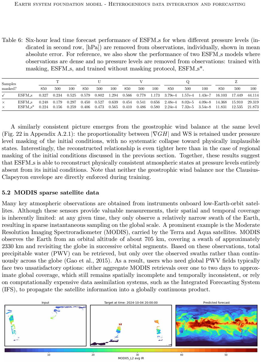
35 25%50% 25% Observation mask verticalmask variable mask spatially for each atmos

URLhttps://proceedings.mlr.press/v162/zhou22g.html. 35 25%50% 25% Observation mask verticalmask variable mask spatially for each atmos. var v; for each vertical l;for each var v; Determine #pixels tomask as N = 0.5xHxW; until N is reached, generate contiguous rectangular masks ofsize 0.2N Figure 20: Schematic of the masking applied to the observations for...

2015
[36]

dataset for time steps between 1979 and

1979
[37]

Accordingly, we have explored variations in the perceiver module, increasing the number of Perceiver blocks, trying newer Perceiver modules, but observed a similar limitation

We suspect that this is due to a limitation of the perceiver module for pressure level aggregation. Accordingly, we have explored variations in the perceiver module, increasing the number of Perceiver blocks, trying newer Perceiver modules, but observed a similar limitation. We will investigate this shortcoming further in the future. 36 Earth system found...

1980
[38]

The training set comprises timeline between start of 1979 and end of

1979
[39]

We select years 2023 and 2024 as the test set

We sample training set randomly and do not actively finetune on the latest years of the training set for any of the experiments. We select years 2023 and 2024 as the test set. Due to prohibitive compute and storage costs, we limit our test set to a subset of these two years. Namely, we pick four weeks that span the year, starting on 02.01, 02.04, 02.07, a...

2023
[40]

In Table 16, we list the full set of variables we have used in this work

The naming convention of the variable abbreviations in CMIP6 differ from ERA5. In Table 16, we list the full set of variables we have used in this work. During training, while the pressure levels of atmospheric variables are 42 Earth system foundation model - Heterogeneous data integration and forecasting Table 12: ERA5 variables used for model training (...

1979
[41]

50, 250, 500, 600, 700, 850, 925 psl zg, ta, hus, ua, va MRI/MRI-ESM2-0 1950–2014NESM3 1.875 (96,

1950
[42]

Dataset Grid res

250, 500, 850 psl ta, ua, va NUIST/NESM3 1950–2014 Table 15: CMPI6 dataset used in the finetuning experiment in Section 5.4.1. Dataset Grid res. [◦] Pixel res. Pressure levels [hPa] Surface vars Atmos vars Full name Time range CNRM 0.5 (360,

1950
[43]

Consequently, the dataset only retains stations with≥90% valid hourly data

50, 250, 500, 600, 700, 850, 925 psl, tos, tws, ci zg, ta, ua, va CNRM-CM6-1-HR 1950–2014 for any remaining missing values. Consequently, the dataset only retains stations with≥90% valid hourly data. ECMWF 11k dataset.Our ECMWF 11k dataset builds upon the source data used by Weather- 5K but introduces significant changes; yielding more samples along time ...

1950
[44]

•Observation filtering.We do not apply spatial or temporal interpolation; all missing values are preserved asNaN

This results in a total of 11’863 stations and 219’168 hourly timesteps. •Observation filtering.We do not apply spatial or temporal interpolation; all missing values are preserved asNaN. This allows keeping station data free from the biases of reanalysis data, which would not be available at test time for station datasets. Raw observations are snapped to ...

2023
[45]

We mapNirregularly spaced weather stations onto aH×Wgrid by wrapping longitudes to [0 ◦,360 ◦), partitioning stations into north-to-south latitude bands and 44 Earth system foundation model - Heterogeneous data integration and forecasting Table 16: CMIP6 variable abbreviations and their full names used in this work. Category Short Name Full Name Surface t...

2023