arxiv: 2605.10395 · v1 · submitted 2026-05-11 · 📊 stat.ML · cond-mat.dis-nn· cond-mat.stat-mech· cs.IT· cs.LG· math.IT

Recognition: 2 theorem links

· Lean Theorem

Sharp feature-learning transitions and Bayes-optimal neural scaling laws in extensive-width networks

Jean Barbier, Minh-Toan Nguyen

Pith reviewed 2026-05-12 02:52 UTC · model grok-4.3

classification 📊 stat.ML cond-mat.dis-nncond-mat.stat-mechcs.ITcs.LGmath.IT

keywords feature learningphase transitionsscaling lawsBayes-optimalteacher-student modelshigh-dimensional regimeeffective widthneural networks

0 comments

The pith

Feature learnability occurs through sharp phase transitions that define an effective width governing Bayes-optimal scaling in wide networks.

A machine-rendered reading of the paper's core claim, the machinery that carries it, and where it could break.

The paper derives closed fixed-point equations for the Bayes-optimal generalization error and individual feature overlaps when learning a one-hidden-layer hierarchical teacher network from noisy data, in the regime where teacher width scales linearly with input dimension. These equations show that features become recoverable sequentially, each through a discontinuous jump in overlap as the number of samples grows, which defines a precise effective width k_c as the number of learnable features at a given data budget. This notion unifies a feature-learning regime where error scales as n to the power 1 over 2 beta minus 1 and a refinement regime scaling as n to the minus 1, both collapsing to the single relation that error is order k_c d over n, where beta is the power-law exponent of the feature hierarchy. The work also shows empirically that Adam-trained students near this effective width nearly match the optimal scaling.

Core claim

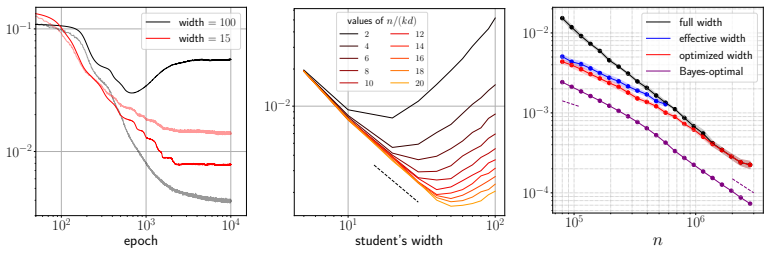
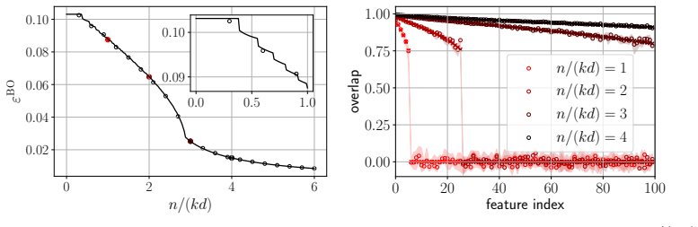
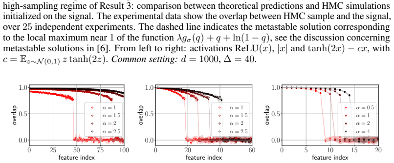
Using a leave-one-out decoupling heuristic, we obtain a system of fixed-point equations for the overlaps and generalization error. These equations exhibit sharp phase transitions where each teacher feature's overlap jumps discontinuously as data n increases, allowing definition of effective width k_c. This leads to the Bayes-optimal error satisfying ε^BO = Θ(k_c d / n), which reproduces the power-law scaling n^{1/(2β)-1} in the feature-learning phase and n^{-1} in the refinement phase for hierarchical features with exponent β.

What carries the argument

The system of closed fixed-point equations from leave-one-out decoupling, which tracks per-feature overlaps and predicts the sequence of sharp transitions that determines effective width k_c.

If this is right

Teacher features are acquired sequentially through discontinuous jumps in overlap as the sample count n increases.
The Bayes-optimal generalization error scales as n to the power 1 over 2 beta minus 1 in the feature-learning regime and as n to the minus 1 in the refinement regime.
Both regimes collapse to the unified scaling ε^BO = Θ(k_c d / n) with k_c the effective width.
A student network trained with Adam near the effective width k_c achieves the information-theoretically optimal scaling laws up to a small algorithmic gap.
Information-theoretic limits on model-size scaling in knowledge transfer follow from the same effective-width relation.

Where Pith is reading between the lines

These are editorial extensions of the paper, not claims the author makes directly.

The sequential transitions suggest that training schedules ordered by feature difficulty could accelerate learning.
Choosing student width near the predicted k_c may minimize the observed algorithmic gap to Bayes optimality.
Similar phase-transition structure may appear in deeper networks or other architectures, yielding analogous effective widths.

Load-bearing premise

The heuristic leave-one-out decoupling argument accurately captures the asymptotic behavior of the Bayes-optimal estimator and feature overlaps.

What would settle it

Numerical computation of the Bayes-optimal estimator in large but finite dimensions that shows feature overlaps varying continuously instead of exhibiting the predicted discontinuous jumps at the critical data sizes.

Figures

Figures reproduced from arXiv: 2605.10395 by Jean Barbier, Minh-Toan Nguyen.

**Figure 1.** Figure 1: ADAM-trained students (all curves except the purple one, right panel) on a teacher with σ(x) = tanh(2x) (with the 2x matching the convention in [6]), k = 100, d = 200, ∆ = 0.01, powerlaw readout with β = 1 (3 batches, 104 epochs, learning rate 0.003; averages over 9 runs, shaded regions show ±1 standard deviation). Left: At fixed sample rate n/(kd) = 2, a reduced-width student (solid = test error; faint =… view at source ↗

**Figure 2.** Figure 2: Bayes-optimal learning curve (left) and feature overlaps at selected values of n/(kd) (right) for σ(x) = tanh(2x), d = 200, k = 100, ∆ = 0.04, power-law readout with β = 0.3. Solid lines and crosses: theoretical predictions from the fixed-point equations (6); circles: averages over 9 independent Hamiltonian Monte Carlo experiments; shaded regions: ±1 standard deviation. Markers on the learning curve indica… view at source ↗

**Figure 3.** Figure 3: Bayes-optimal overlap as a function of the SNR [PITH_FULL_IMAGE:figures/full_fig_p020_3.png] view at source ↗

**Figure 4.** Figure 4: Bayes-optimal feature overlaps in the neural network model [PITH_FULL_IMAGE:figures/full_fig_p020_4.png] view at source ↗

read the original abstract

We study the information-theoretic limits of learning a one-hidden-layer teacher network with hierarchical features from noisy queries, in the context of knowledge transfer to a smaller student model. We work in the high-dimensional regime where the teacher width $k$ scales linearly with the input dimension $d$ -- a setting that captures large-but-finite-width networks and has only recently become analytically tractable. Using a heuristic leave-one-out decoupling argument, validated numerically throughout, we derive asymptotically sharp characterizations of the Bayes-optimal generalization error and individual feature overlaps via a system of closed fixed-point equations. These equations reveal that feature learnability is governed by a sequence of sharp phase transitions: as data grows, teacher features become recoverable sequentially, each through a discontinuous jump in overlap. This sequential acquisition underlies a precise notion of \textit{effective width} $k_c$ -- the number of learnable features at a given data budget $n$ -- which unifies two distinct scaling regimes: a feature-learning regime in which the Bayes-optimal generalization error $\varepsilon^{\rm BO}$ scales as $ n^{1/(2\beta)-1}$, and a refinement regime in which it scales as $n^{-1}$, where $\beta>1/2$ is the exponent of the power-law feature hierarchy. Both laws collapse to the single relation $\varepsilon^{\rm BO}=\Theta(k_c d/n)$. We further show empirically that a student trained with \textsc{Adam} near the effective width $k_c$ achieves these optimal scaling laws (up to a small algorithmic gap), and provide an information-theoretic account of the associated scaling in model size.

Editorial analysis

A structured set of objections, weighed in public.

Desk editor's note, referee report, simulated authors' rebuttal, and a circularity audit. Tearing a paper down is the easy half of reading it; the pith above is the substance, this is the friction.

Desk Editor's Note private letter to a colleague

The paper gives a heuristic derivation of sequential sharp feature transitions in extensive-width nets that collapses scaling laws via an effective width, but the decoupling step needs more scrutiny to confirm the discontinuities survive in the limit.

read the letter

The central claim is that a leave-one-out decoupling produces closed fixed-point equations for feature overlaps and Bayes-optimal error, revealing that teacher features recover one by one through discontinuous jumps as n grows. This defines an effective width k_c that unifies a feature-learning regime scaling as n to the power 1/(2 beta) minus 1 with a refinement regime scaling as n to the minus 1, both reducing to epsilon_BO equals Theta of k_c d over n. The numerical checks on finite instances line up with the equations, and the Adam student experiments show the scaling is nearly achieved in practice. That unification and the sequential-transition picture are the genuinely new pieces in the extensive-width regime. The derivation is internally consistent and the connection to practical training is useful. The main limitation is that the decoupling remains heuristic. When k scales linearly with d, collective correlations could persist and either smooth the jumps or shift their locations, which would change how sharply the scaling collapses. The paper validates numerically but does not supply a rigorous error bound or alternative derivation that would confirm the transitions stay discontinuous in the thermodynamic limit. This work is for theorists who track statistical-physics approaches to scaling and feature learning. Readers who want concrete predictions for when specific features become recoverable will find the fixed-point system and k_c concept worth examining. It deserves peer review because the regime matches practical large models and the results are coherent under the stated assumptions, even with the heuristic caveat. I would send it out and ask the authors to discuss the approximation's potential failure modes more explicitly.

Referee Report

2 major / 2 minor

Summary. The paper studies the information-theoretic limits of learning a one-hidden-layer teacher network with hierarchical features (power-law exponent β) from noisy queries in the extensive-width regime where teacher width k scales linearly with input dimension d. Using a heuristic leave-one-out decoupling argument that is numerically validated, the authors derive closed fixed-point equations characterizing the Bayes-optimal generalization error ε^BO and individual feature overlaps. These reveal a sequence of sharp phase transitions in feature recoverability, leading to an effective width k_c (number of learnable features at data budget n) that unifies a feature-learning scaling regime ε^BO ~ n^{1/(2β)-1} and a refinement regime ε^BO ~ n^{-1}, both collapsing to ε^BO = Θ(k_c d/n). Empirical results show that Adam-trained students near k_c achieve these laws up to a small gap.

Significance. If the decoupling heuristic becomes exact in the thermodynamic limit, the work provides a precise, non-asymptotic-in-width characterization of optimal feature learning and scaling laws in high-dimensional networks, including the novel notion of effective width unifying regimes. The closed fixed-point equations, numerical validation of transitions, and empirical match with practical optimization are notable strengths that could inform both theory and algorithm design for hierarchical data.

major comments (2)

[heuristic leave-one-out decoupling argument and fixed-point equations] The central derivation of the fixed-point equations for overlaps and ε^BO (detailed after the abstract) rests on a heuristic leave-one-out decoupling argument. While the manuscript numerically validates the resulting phase transitions and scaling collapse on finite instances, it does not establish that residual feature correlations vanish in the k ~ d limit, which is required for the claimed discontinuous jumps in overlap and the sharpness of k_c. This is load-bearing for the unification of the two scaling regimes.
[effective width k_c and scaling collapse] The effective width k_c is defined from the solved overlaps, and the collapse ε^BO = Θ(k_c d/n) is asserted to hold across regimes. However, the manuscript does not provide an explicit derivation of the proportionality constant or error bounds showing that collective effects do not shift the transition points when k scales linearly with d.

minor comments (2)

[model definition] The power-law exponent β is introduced in the abstract but its precise definition in the teacher network (e.g., how feature strengths decay) could be stated explicitly in the model setup for immediate clarity.
[numerical results] Figure captions or legends for the numerical validations of the phase transitions should include the specific values of d, k, and β used, to facilitate direct comparison with the fixed-point predictions.

Simulated Author's Rebuttal

2 responses · 2 unresolved

We thank the referee for their careful reading and constructive comments, which highlight important aspects of our heuristic approach. We address each major comment below, providing clarifications on the scope of our results while remaining faithful to the manuscript's content and limitations.

read point-by-point responses

Referee: The central derivation of the fixed-point equations for overlaps and ε^BO (detailed after the abstract) rests on a heuristic leave-one-out decoupling argument. While the manuscript numerically validates the resulting phase transitions and scaling collapse on finite instances, it does not establish that residual feature correlations vanish in the k ~ d limit, which is required for the claimed discontinuous jumps in overlap and the sharpness of k_c. This is load-bearing for the unification of the two scaling regimes.

Authors: We agree that the derivation relies on a heuristic leave-one-out decoupling argument, which assumes that residual correlations between features become negligible in the extensive-width limit. The manuscript explicitly describes this as heuristic and supports it through extensive numerical validation of the phase transitions and fixed-point predictions on finite instances. We do not claim or provide a rigorous proof that correlations vanish exactly when k scales linearly with d. In a revision, we will add further discussion emphasizing the heuristic character, the numerical evidence for correlation decay, and the conditions under which the decoupling is expected to hold. revision: partial
Referee: The effective width k_c is defined from the solved overlaps, and the collapse ε^BO = Θ(k_c d/n) is asserted to hold across regimes. However, the manuscript does not provide an explicit derivation of the proportionality constant or error bounds showing that collective effects do not shift the transition points when k scales linearly with d.

Authors: The scaling relation ε^BO = Θ(k_c d/n) is obtained by substituting the solved overlaps into the expression for the Bayes-optimal error, where each unrecovered feature contributes an additive term of order d/n. The leading proportionality follows directly from this structure in the high-dimensional regime. We acknowledge that the manuscript does not supply a rigorous derivation of the constant or error bounds that fully control collective effects at k ~ d. Our numerical experiments with k proportional to d nevertheless show the collapse holds with only small deviations. In revision, we will include an expanded heuristic derivation of the Θ scaling and additional discussion of its robustness. revision: partial

standing simulated objections not resolved

A rigorous proof that residual feature correlations vanish in the k ~ d limit, which would be needed to establish the discontinuous jumps and sharpness of k_c without relying on the heuristic.
An explicit derivation of the proportionality constant together with error bounds for the scaling collapse that account for possible collective effects when k scales linearly with d.

Circularity Check

0 steps flagged

No circularity: derivation proceeds from heuristic decoupling to independent fixed-point equations and derived quantities

full rationale

The paper derives closed fixed-point equations for overlaps and Bayes-optimal error via a leave-one-out decoupling argument (explicitly labeled heuristic and numerically validated). From these equations it extracts sequential phase transitions, defines effective width k_c as the count of features with positive overlap, and obtains the two scaling regimes that collapse to ε^BO = Θ(k_c d/n). None of these steps is self-definitional, a fitted input renamed as prediction, or dependent on self-citation; the fixed-point system is not tautological with the target scaling laws, and k_c is a post-hoc counting function of the solved overlaps rather than an input parameter. The analysis is therefore self-contained against external benchmarks.

Axiom & Free-Parameter Ledger

0 free parameters · 1 axioms · 0 invented entities

The analysis depends on the validity of the leave-one-out heuristic in the high-dimensional limit with k scaling linearly with d; no free parameters are explicitly fitted beyond the given power-law exponent β>1/2 for the feature hierarchy.

axioms (1)

domain assumption The leave-one-out decoupling argument provides asymptotically sharp characterizations of overlaps and generalization error in the extensive-width regime
Invoked to close the system of fixed-point equations for Bayes-optimal quantities.

pith-pipeline@v0.9.0 · 5591 in / 1477 out tokens · 70724 ms · 2026-05-12T02:52:33.859804+00:00 · methodology

discussion (0)

Lean theorems connected to this paper

Citations machine-checked in the Pith Canon. Every link opens the source theorem in the public Lean library.

IndisputableMonolith/Cost/FunctionalEquation.lean washburn_uniqueness_aczel unclear
qi = m_σ(n v_i²/d/(Δ+ε)), ε = ∑ v_i² (g_σ(1)−g_σ(q_i)) with m_σ(λ) = argmax [λ g_σ(q) + q + ln(1−q)]
IndisputableMonolith/Foundation/RealityFromDistinction.lean reality_from_one_distinction unclear
sharp staircase of feature-learning transitions … effective width k_c … ε^BO = Θ(k_c d/n)

Reference graph

Works this paper leans on

54 extracted references · 54 canonical work pages · 4 internal anchors

[1]

Sgd learning on neural net- works: leap complexity and saddle-to-saddle dynamics

Emmanuel Abbe, Enric Boix Adsera, and Theodor Misiakiewicz. Sgd learning on neural net- works: leap complexity and saddle-to-saddle dynamics. InThe Thirty Sixth Annual Conference on Learning Theory, pages 2552–2623. PMLR, 2023

work page 2023
[2]

Learning quadratic neural networks in high dimensions: SGD dynamics and scaling laws.arXiv preprint arXiv:2508.03688, 2025

Gérard Ben Arous, Murat A Erdogdu, N Mert Vural, and Denny Wu. Learning quadratic neural networks in high dimensions: Sgd dynamics and scaling laws.arXiv preprint arXiv:2508.03688, 2025

work page arXiv 2025
[3]

Online stochastic gradient descent on non-convex losses from high-dimensional inference.Journal of Machine Learning Research, 22(106):1–51, 2021

Gerard Ben Arous, Reza Gheissari, and Aukosh Jagannath. Online stochastic gradient descent on non-convex losses from high-dimensional inference.Journal of Machine Learning Research, 22(106):1–51, 2021

work page 2021
[4]

The committee machine: Computational to statistical gaps in learning a two-layers neural network.Advances in Neural Information Processing Systems, 31, 2018

Benjamin Aubin, Antoine Maillard, Florent Krzakala, Nicolas Macris, Lenka Zdeborová, et al. The committee machine: Computational to statistical gaps in learning a two-layers neural network.Advances in Neural Information Processing Systems, 31, 2018

work page 2018
[5]

Explaining neural scaling laws.Proceedings of the National Academy of Sciences, 121(27):e2311878121, 2024

Yasaman Bahri, Ethan Dyer, Jared Kaplan, Jaehoon Lee, and Utkarsh Sharma. Explaining neural scaling laws.Proceedings of the National Academy of Sciences, 121(27):e2311878121, 2024

work page 2024
[6]

Statisti- cal physics of deep learning: Optimal learning of a multi-layer perceptron near interpolation

Jean Barbier, Francesco Camilli, Minh-Toan Nguyen, Mauro Pastore, and Rudy Skerk. Statisti- cal physics of deep learning: Optimal learning of a multi-layer perceptron near interpolation. Physical Review X, Apr 2026

work page 2026
[7]

Optimal errors and phase transitions in high-dimensional generalized linear models.Proceedings of the National Academy of Sciences, 116(12):5451–5460, 2019

Jean Barbier, Florent Krzakala, Nicolas Macris, Léo Miolane, and Lenka Zdeborová. Optimal errors and phase transitions in high-dimensional generalized linear models.Proceedings of the National Academy of Sciences, 116(12):5451–5460, 2019

work page 2019
[8]

Strong replica symmetry in high-dimensional optimal bayesian inference.Communications in mathematical physics, 393(3):1199–1239, 2022

Jean Barbier and Dmitry Panchenko. Strong replica symmetry in high-dimensional optimal bayesian inference.Communications in mathematical physics, 393(3):1199–1239, 2022

work page 2022
[9]

The dynamics of message passing on dense graphs, with applications to compressed sensing.IEEE Transactions on Information Theory, 57(2):764–785, 2011

Mohsen Bayati and Andrea Montanari. The dynamics of message passing on dense graphs, with applications to compressed sensing.IEEE Transactions on Information Theory, 57(2):764–785, 2011

work page 2011
[10]

A dynamical model of neural scaling laws

Blake Bordelon, Alexander Atanasov, and Cengiz Pehlevan. A dynamical model of neural scaling laws. InInternational Conference on Machine Learning, pages 4345–4382. PMLR, 2024

work page 2024
[11]

Model compression

Cristian Bucilu ˇa, Rich Caruana, and Alexandru Niculescu-Mizil. Model compression. In Proceedings of the 12th ACM SIGKDD international conference on Knowledge discovery and data mining, pages 535–541, 2006

work page 2006
[12]

Learning curves theory for hierarchi- cally compositional data with power-law distributed features.arXiv preprint arXiv:2505.07067, 2025

Francesco Cagnetta, Hyunmo Kang, and Matthieu Wyart. Learning curves theory for hierarchi- cally compositional data with power-law distributed features.arXiv preprint arXiv:2505.07067, 2025

work page arXiv 2025
[13]

Information-theoretic reduction of deep neural networks to linear models in the overparametrized proportional regime

Francesco Camilli, Daria Tieplova, Eleonora Bergamin, and Jean Barbier. Information-theoretic reduction of deep neural networks to linear models in the overparametrized proportional regime. InThe Thirty Eighth Annual Conference on Learning Theory, pages 757–798. PMLR, 2025

work page 2025
[14]

On lazy training in differentiable program- ming.Advances in neural information processing systems, 32, 2019

Lenaic Chizat, Edouard Oyallon, and Francis Bach. On lazy training in differentiable program- ming.Advances in neural information processing systems, 32, 2019. 10

work page 2019
[15]

Generalization error rates in kernel regression: The crossover from the noiseless to noisy regime.Advances in Neural Information Processing Systems, 34:10131–10143, 2021

Hugo Cui, Bruno Loureiro, Florent Krzakala, and Lenka Zdeborová. Generalization error rates in kernel regression: The crossover from the noiseless to noisy regime.Advances in Neural Information Processing Systems, 34:10131–10143, 2021

work page 2021
[16]

Smoothing the landscape boosts the signal for sgd: Optimal sample complexity for learning single index models.Advances in Neural Information Processing Systems, 36:752–784, 2023

Alex Damian, Eshaan Nichani, Rong Ge, and Jason D Lee. Smoothing the landscape boosts the signal for sgd: Optimal sample complexity for learning single index models.Advances in Neural Information Processing Systems, 36:752–784, 2023

work page 2023
[17]

Computational-statistical gaps in gaussian single-index models

Alex Damian, Loucas Pillaud-Vivien, Jason Lee, and Joan Bruna. Computational-statistical gaps in gaussian single-index models. InThe Thirty Seventh Annual Conference on Learning Theory, pages 1262–1262. PMLR, 2024

work page 2024
[18]

Neural networks can learn represen- tations with gradient descent

Alexandru Damian, Jason Lee, and Mahdi Soltanolkotabi. Neural networks can learn represen- tations with gradient descent. InConference on Learning Theory, pages 5413–5452. PMLR, 2022

work page 2022
[19]

A noise sensitiv- ity exponent controls large statistical-to-computational gaps in single-and multi-index models

Leonardo Defilippis, Florent Krzakala, Bruno Loureiro, and Antoine Maillard. A noise sensitiv- ity exponent controls large statistical-to-computational gaps in single-and multi-index models. arXiv preprint arXiv:2603.17896, 2026

work page arXiv 2026
[20]

Optimal scaling laws in learning hierarchical multi-index models.arXiv preprint arXiv:2602.05846, 2026

Leonardo Defilippis, Florent Krzakala, Bruno Loureiro, and Antoine Maillard. Optimal scaling laws in learning hierarchical multi-index models.arXiv preprint arXiv:2602.05846, 2026

work page arXiv 2026
[21]

Dimension-free deterministic equivalents and scaling laws for random feature regression.Advances in Neural Information Processing Systems, 37:104630–104693, 2024

Leonardo Defilippis, Bruno Loureiro, and Theodor Misiakiewicz. Dimension-free deterministic equivalents and scaling laws for random feature regression.Advances in Neural Information Processing Systems, 37:104630–104693, 2024

work page 2024
[22]

Scaling laws and spectra of shallow neural networks in the feature learning regime.arXiv preprint arXiv:2509.24882, 2025

Leonardo Defilippis, Yizhou Xu, Julius Girardin, Emanuele Troiani, Vittorio Erba, Lenka Zdeborová, Bruno Loureiro, and Florent Krzakala. Scaling laws and spectra of shallow neural networks in the feature learning regime.arXiv preprint arXiv:2509.24882, 2025

work page arXiv 2025
[23]

An exactly solvable model for emergence and scaling laws in the multitask sparse parity problem.Advances in Neural Information Processing Systems, 37:39632–39693, 2024

Nayara Fonseca, Seok Hyeong Lee, Chris Mingard, Ard Louis, et al. An exactly solvable model for emergence and scaling laws in the multitask sparse parity problem.Advances in Neural Information Processing Systems, 37:39632–39693, 2024

work page 2024
[24]

Linearized two-layers neural networks in high dimension.The Annals of Statistics, 49(2):1029–1054, 2021

Behrooz Ghorbani, Song Mei, Theodor Misiakiewicz, and Andrea Montanari. Linearized two-layers neural networks in high dimension.The Annals of Statistics, 49(2):1029–1054, 2021

work page 2021
[25]

Knowledge distillation: A survey.International journal of computer vision, 129(6):1789–1819, 2021

Jianping Gou, Baosheng Yu, Stephen J Maybank, and Dacheng Tao. Knowledge distillation: A survey.International journal of computer vision, 129(6):1789–1819, 2021

work page 2021
[26]

Deep Learning Scaling is Predictable, Empirically

Joel Hestness, Sharan Narang, Newsha Ardalani, Gregory Diamos, Heewoo Jun, Hassan Kianinejad, Md Mostofa Ali Patwary, Yang Yang, and Yanqi Zhou. Deep learning scaling is predictable, empirically.arXiv preprint arXiv:1712.00409, 2017

work page internal anchor Pith review arXiv 2017
[27]

Distilling the Knowledge in a Neural Network

Geoffrey Hinton, Oriol Vinyals, and Jeff Dean. Distilling the knowledge in a neural network. arXiv preprint arXiv:1503.02531, 2015

work page internal anchor Pith review Pith/arXiv arXiv 2015
[28]

Training Compute-Optimal Large Language Models

Jordan Hoffmann, Sebastian Borgeaud, Arthur Mensch, Elena Buchatskaya, Trevor Cai, Eliza Rutherford, DDL Casas, Lisa Anne Hendricks, Johannes Welbl, Aidan Clark, et al. Training compute-optimal large language models.arXiv preprint arXiv:2203.15556, 10, 2022

work page internal anchor Pith review Pith/arXiv arXiv 2022
[29]

Learning curve theory.arXiv preprint arXiv:2102.04074, 2021

Marcus Hutter. Learning curve theory.arXiv preprint arXiv:2102.04074, 2021

work page arXiv 2021
[30]

Neural tangent kernel: Convergence and generalization in neural networks.Advances in neural information processing systems, 31, 2018

Arthur Jacot, Franck Gabriel, and Clément Hongler. Neural tangent kernel: Convergence and generalization in neural networks.Advances in neural information processing systems, 31, 2018

work page 2018
[31]

Scaling Laws for Neural Language Models

Jared Kaplan, Sam McCandlish, Tom Henighan, Tom B Brown, Benjamin Chess, Rewon Child, Scott Gray, Alec Radford, Jeffrey Wu, and Dario Amodei. Scaling laws for neural language models.arXiv preprint arXiv:2001.08361, 2020. 11

work page internal anchor Pith review Pith/arXiv arXiv 2001
[32]

Scaling laws in linear regression: Compute, parameters, and data.Advances in Neural Information Processing Systems, 37:60556–60606, 2024

Licong Lin, Jingfeng Wu, Sham M Kakade, Peter L Bartlett, and Jason D Lee. Scaling laws in linear regression: Compute, parameters, and data.Advances in Neural Information Processing Systems, 37:60556–60606, 2024

work page 2024
[33]

Bayes-optimal learning of an extensive-width neural network from quadratically many samples

Antoine Maillard, Emanuele Troiani, Simon Martin, Lenka Zdeborová, and Florent Krzakala. Bayes-optimal learning of an extensive-width neural network from quadratically many samples. Advances in Neural Information Processing Systems, 37:82085–82132, 2024

work page 2024
[34]

The quantization model of neural scaling.Advances in Neural Information Processing Systems, 36:28699–28722, 2023

Eric Michaud, Ziming Liu, Uzay Girit, and Max Tegmark. The quantization model of neural scaling.Advances in Neural Information Processing Systems, 36:28699–28722, 2023

work page 2023
[35]

4+ 3 phases of compute-optimal neural scaling laws.Advances in Neural Information Processing Systems, 37:16459–16537, 2024

Elliot Paquette, Courtney Paquette, Lechao Xiao, and Jeffrey Pennington. 4+ 3 phases of compute-optimal neural scaling laws.Advances in Neural Information Processing Systems, 37:16459–16537, 2024

work page 2024
[36]

Emergence and scaling laws in sgd learning of shallow neural networks.arXiv preprint arXiv:2504.19983, 2025

Yunwei Ren, Eshaan Nichani, Denny Wu, and Jason D Lee. Emergence and scaling laws in sgd learning of shallow neural networks.arXiv preprint arXiv:2504.19983, 2025

work page arXiv 2025
[37]

Springer Science & Business Media, 2010

Michel Talagrand.Mean field models for spin glasses: Volume I: Basic examples, volume 54. Springer Science & Business Media, 2010

work page 2010
[38]

Fundamental computational limits of weak learnability in high-dimensional multi-index models

Emanuele Troiani, Yatin Dandi, Leonardo Defilippis, Lenka Zdeborova, Bruno Loureiro, and Florent Krzakala. Fundamental computational limits of weak learnability in high-dimensional multi-index models. InInternational Conference on Artificial Intelligence and Statistics, pages 2467–2475. PMLR, 2025

work page 2025
[39]

replica symmetric potential

Ge Yang, Edward Hu, Igor Babuschkin, Szymon Sidor, Xiaodong Liu, David Farhi, Nick Ryder, Jakub Pachocki, Weizhu Chen, and Jianfeng Gao. Tuning large neural networks via zero-shot hyperparameter transfer.Advances in Neural Information Processing Systems, 34:17084–17097, 2021. 12 A Hermite expansion and information exponent Theℓ-th Hermite polynomial is de...

work page 2021
[40]

4.g ′ σ =g σ′

If k⋆(σ)≥3 , there exists λσ >0 , qσ >0 such that mσ(λ) = 0 if λ < λ σ and limλ→λ+ σ mσ(λ) =q σ. 4.g ′ σ =g σ′. Proof. 1. RecallMehler’s formula: for (z1, z2) a centered Gaussian vector with unit variances and correlationx∈[−1,1], E[Heℓ(z1)Hem(z2)] =δ ℓm ℓ!x ℓ, ℓ, m≥0.(27) Writing σ= P ℓ≥0 µℓ ℓ! Heℓ in L2(µ) and using the orthogonality (27), we obtain, fo...

work page
[41]

Monotonicity.Considerλ 1 > λ2 ≥0

Recall that mσ(λ) = arg max q∈[0,1) F(λ, q), F(λ, q) =λg σ(q) +q+ ln(1−q). Monotonicity.Considerλ 1 > λ2 ≥0. Letq 1 =m σ(λ1),q 2 =m σ(λ2). By optimality ofq 1 andq 2, F(λ 1, q1)≥F(λ 1, q2), F(λ 2, q2)≥F(λ 2, q1). Adding the two inequalities and simplifying, (λ1 −λ 2) gσ(q1)−g σ(q2) ≥0. Since λ1 > λ 2, this implies gσ(q1)≥g σ(q2). Since gσ is strictly incr...

work page
[42]

Indeed, we have ∂2 q F(λ, q) =λg ′′ σ(q)− 1 (1−q) 2 , which gives ∂2 q=0F(λ, q) =−1<0 , since g′′ σ(0) = 0 as k⋆(σ)≥3

We first observe that q= 0 is always a local maximum of F(λ, q) for every λ≥0 . Indeed, we have ∂2 q F(λ, q) =λg ′′ σ(q)− 1 (1−q) 2 , which gives ∂2 q=0F(λ, q) =−1<0 , since g′′ σ(0) = 0 as k⋆(σ)≥3 . Next, q= 0 is the global maximum if and only if λgσ(q) +q+ ln(1−q)<0,∀q∈(0,1), which is equivalent to λ < λ σ := inf q∈(0,1) h(q), h(q) = −q−ln(1−q) gσ(q) .(...

work page
[43]

off-diagonal

Expand σ(z) = X ℓ≥0 aℓHeℓ(z), a ℓ =µ ℓ/ℓ!. Using He′ ℓ(z) =ℓHe ℓ−1(z) and the assumption σ′ ∈L 2(µ) (so the term-by-term differentiation is justified inL 2), we obtain σ′(z) = X ℓ≥1 aℓℓHe ℓ−1(z). Mehler’s formula gives E[Heℓ(z1)Hem(z2)] =δ ℓm ℓ!x ℓ for(z 1, z2)∼ N 0, " 1x x1 #! . 16 Therefore, gσ(x) =E[σ(z 1)σ(z2)] = X ℓ≥0 a2 ℓ ℓ!x ℓ, so g′ σ(x) = X ℓ≥1 a...

work page
[44]

This identity is useful for bounding B when n is very large, as in this regime the overlapsQ ii ≃q i are close to1, which suppresses the off-diagonal terms

P i Q2 ij =P j Q2 ij = 1. This identity is useful for bounding B when n is very large, as in this regime the overlapsQ ii ≃q i are close to1, which suppresses the off-diagonal terms

work page
[45]

Var(B)≲ X i̸=j v2 i v2 j Var(Q3 ij), This improves upon the pessimistic upper bound we used in the dense readout, interpolation regime

Experimentally, we observe thatQ ij fori̸=jareasymptotically uncorrelated, i.e. Var(B)≲ X i̸=j v2 i v2 j Var(Q3 ij), This improves upon the pessimistic upper bound we used in the dense readout, interpolation regime. G Optimal scaling laws forβ >1/2 Recall that the effective SNR for featureiis snri = (n/d)v2 i ∆ +ε BO . Consequently, the weakest feature (i...

work page
[46]

Letα c(v) = sup{α≥0 :Q(v) = 0}, then αc(v) = 1 v2 λσγ ∆ +g σ(1)−E v∼Pv h v2gσ ◦m σ λσv2 v2 i . 20 In particular, if maxi vi converges to a limiting value vmax, then the first phase transition– corresponding to the feature with the largest readout–occurs at α= λσγ(∆ +g σ(1)) v2max .(36) Proof.1. Fixi∈I v,δ, we have (v−δ) 2 k ≤v 2 i ≤ (v+δ) 2 k Therefore, n...

work page
[47]

From the definition of αc(v) and equation (37), using the fact that λσ = sup{λ≥0 :m σ(λ) = 0}, we have αc(v)v2 ∆ +ε =λ σ. Therefore, αc(v) = 1 v2 λσγ(∆ +ε) = 1 v2 λσγ(∆ +g σ(1)−E v∼Pv[v2gσ ◦ Q(v)]) = 1 v2 λσγ ∆ +g σ(1)−E v∼Pv h v2gσ ◦m σ αc(v)v2 γ(∆ +ε) i = 1 v2 λσγ ∆ +g σ(1)−E v∼Pv h v2gσ ◦m σ λσv2 v2 i If v=v max, then for any v∈supp(P v), we have λσv2/...

work page
[48]

Ifk c < kandi=⌊xk c⌋for somex∈(0,1), then lim d→∞ qi =m σ(λσx−2β) :=ϕ(x)(39) In other words, the overlaps (qi)k i=1 in the infinite dimension limit can be compactly described by a limiting profileϕ

work page
[49]

Forβ >1/2, let ¯kc = lim d→∞ kcd− 1 2β ,¯ε BO = lim d→∞ εBOd− 1 2β +1,(40) Then, lettingz(β) := P∞ i=1 i−2β and sinceε= 0, ¯kc = α λσz(β)∆ 1 2β (41) ¯εBO = ¯k1−2β c z(β) Z 1 0 gσ(1)−g σ(ϕ(x)) x2β dx+ gσ(1) (2β−1) .(42)

work page
[50]

We have nv2 kc+1 d(∆ +ε BO) < λ σ < nv2 kc d(∆ +ε BO) .(47) From the inequality on the left, it is clear thatkc → ∞ as d→ ∞

Forβ <1/2, let ¯kc = lim d→∞ kc/k, ε= lim d→∞ εBO.(43) Thenεis the unique solution in(0,∞)of gσ(1)−ε 1−2β = Z 1 0 x−2βgσ ◦m σ α(1−2β) γ(∆ +ε) x−2β dx(44) and ¯kc = (1−2β)α λσγ(∆ +ε) 1 2β (45) Moreover, in the thermodynamic limit, all features are learnable if and only if α > α ⋆, where α⋆ λσγ = ∆ +g σ(1) 1−2β − Z 1 0 gσ(ϕ(x)) x2β dx,(46) Derivation.1. We ...

work page
[51]

From (48), straightforward calculations yield lim d→∞ kc d− 1 2β = α λσz(β)(∆ +ε) 1 2β .(52) Next, usingq i ≃ϕ(i/k c)fori≤k c, the error contributed by learnable features is X i≤kc i−2β z(β) (gσ(1)−g σ ◦ϕ(i/k c)) =k 1−2β c 1 kc X i≤kc (i/kc)−2β z(β) (gσ(1)−g σ ◦ϕ(i/k c))(53) ≃k 1−2β c Z 1 0 x−2β z(β) (gσ(1)−g σ(ϕ(x)))dx.(54) where in the last step, averag...

work page
[52]

Let us denote α⋆ = lim d→∞ αc(k)(58) where we recall that αc(k) is the threshold of α for the feature k to be learnable

We have v2 i = i−2β Pk j=1 j−2β ≃(1−2β)i −2βk2β−1 (56) From (48), straightforward calculations yield lim d→∞ kc/k= (1−2β)α λσγ(∆ +ε) 1 2β (57) In this case it is possible for all features to be learnable. Let us denote α⋆ = lim d→∞ αc(k)(58) where we recall that αc(k) is the threshold of α for the feature k to be learnable. Let ε be the BO error at this v...

work page
[53]

The student’s features are normalized after each epoch, preventing their norms from growing excessively and resulting in more stable and well-behaved training dynamics

work page
[54]

Performance degrades when the student’s readout is fixed to match the teacher during training, as the student is more likely to get stuck in local minima. In contrast, when the student readout is learnable, it still recovers that of the teacher, and the possibility for the readout to change during training helps the student escape local minima. 25

work page