Recognition: 2 theorem links
· Lean TheoremSteering Without Breaking: Mechanistically Informed Interventions for Discrete Diffusion Language Models
Pith reviewed 2026-05-13 06:39 UTC · model grok-4.3
The pith
Adaptive timing of interventions based on attribute formation schedules improves steering strength in discrete diffusion language models without degrading quality.
A machine-rendered reading of the paper's core claim, the machinery that carries it, and where it could break.
Core claim
Different attributes in discrete diffusion language models commit on distinct schedules during the parallel denoising process, varying in timing, sharpness, and magnitude. Selectively intervening only on the steps where a target attribute is actively forming, using schedules recovered by sparse autoencoders, achieves precise control without the quality degradation that uniform interventions produce.
What carries the argument
Sparse autoencoder-derived commitment schedules that identify the specific denoising steps where each attribute forms.
If this is right
- The performance advantage of adaptive over uniform scheduling is governed by a single dispersion statistic of the commitment distribution.
- On simultaneous three-attribute control tasks, steering strength reaches up to 93 percent and exceeds the strongest baseline by up to 15 points.
- Generation quality is preserved across both single-attribute and multi-attribute steering.
- The method applies consistently to discrete diffusion models ranging from 124 million to 8 billion parameters.
Where Pith is reading between the lines
- Similar timing-based intervention strategies may improve steering performance in other non-autoregressive generation frameworks.
- Sparse autoencoders could serve as a general tool for discovering optimal intervention windows in diffusion-based text models.
- Reliable multi-attribute control could support downstream applications that require simultaneous constraints on topic, sentiment, and style.
Load-bearing premise
The commitment schedules recovered by sparse autoencoders accurately reflect when each attribute forms during denoising.
What would settle it
Running the adaptive scheduler on a new model or attribute set where the recovered schedules are deliberately shifted by a fixed number of steps and observing no gain in steering strength or quality would falsify the claim.
Figures


read the original abstract
Discrete diffusion language models (DLMs) generate text by iteratively denoising all positions in parallel, offering an alternative to autoregressive models. Controlled generation methods for DLMs, imported from autoregressive models, apply uniform intervention at every denoising steps. We show this uniform schedule degrades quality, and the damage compounds when multiple attributes are steered jointly. To diagnose the failure, we train sparse autoencoders on four DLMs (124M-8B parameters) and find that different attributes commit on distinct schedules, varying in timing, sharpness, and magnitude. For instance, topic commits within the first 2\% of denoising, whereas sentiment emerges gradually over 20\% of the process. Consequently, uniform intervention wastes steering capacity on steps where the target attribute has already solidified or has yet to emerge. We propose a novel adaptive scheduler that concentrates interventions on the steps where an attribute is actively forming and leaves the rest of generation untouched. The cost-control trade-off admits a closed-form characterization: the advantage of adaptive over uniform scheduling is governed by a single dispersion statistic of the commitment distribution. Across four DLMs and seven steering tasks, our method achieves precise control without the degradation typical of uniform interventions. Especially on challenging simultaneous three-attribute control, it reaches up to 93\% steering strength, beating the strongest baseline by up to 15\% points while preserving generation quality.
Editorial analysis
A structured set of objections, weighed in public.
Referee Report
Summary. The manuscript proposes an adaptive scheduler for steering discrete diffusion language models (DLMs) based on sparse autoencoder (SAE) analysis of attribute commitment during denoising. It argues that uniform interventions degrade quality, especially in multi-attribute control, and that concentrating interventions on steps where attributes are forming—identified via SAE features—achieves better control with less degradation. A closed-form characterization of the advantage is provided in terms of a dispersion statistic of the commitment distribution, supported by experiments on four model sizes and seven tasks showing up to 93% steering strength and 15% improvement over baselines.
Significance. If the SAE-derived commitment schedules accurately capture causal formation dynamics, this work offers a principled method for controlled generation in DLMs that avoids the quality trade-offs of uniform approaches. The closed-form characterization could provide a general tool for analyzing intervention schedules, and the empirical results suggest practical gains in multi-attribute steering while maintaining generation quality.
major comments (3)
- [Abstract] Abstract: The reported gains (up to 15 percentage points on three-attribute control) are presented without error bars, statistical significance tests, or ablation details on SAE feature selection and intervention timing, which undermines assessment of robustness across the four model sizes and seven tasks.
- [§3] §3 (SAE analysis): The central assumption that SAE feature activations identify the causal windows where intervention is necessary and sufficient for attribute control is load-bearing for the adaptive scheduler's claimed isolation from other attributes and generation dynamics; if activations instead reflect downstream correlations, the selected steps would not be minimal and the advantage over uniform schedules would not hold.
- [Closed-form characterization] Closed-form characterization: The advantage is governed by a dispersion statistic of the commitment distribution, but the manuscript does not demonstrate that this statistic is independent of SAE training choices or that the schedule remains effective when attribute information is distributed across multiple features rather than the sparse subset used.
minor comments (2)
- [Notation] Notation in the commitment distribution definition should explicitly state how the dispersion statistic is computed from SAE activations to allow reproduction.
- [Figures] Figures showing commitment schedules over denoising steps would benefit from overlays of multiple runs or variance bands to illustrate stability of the recovered timings.
Simulated Author's Rebuttal
We thank the referee for their constructive comments. We address each of the major comments below, indicating the revisions we plan to make to strengthen the manuscript.
read point-by-point responses
-
Referee: [Abstract] Abstract: The reported gains (up to 15 percentage points on three-attribute control) are presented without error bars, statistical significance tests, or ablation details on SAE feature selection and intervention timing, which undermines assessment of robustness across the four model sizes and seven tasks.
Authors: We agree that including error bars, statistical tests, and ablation details would improve the assessment of our results. In the revised manuscript, we will add error bars to all reported figures and tables, include statistical significance tests (e.g., paired t-tests) for the gains over baselines, and expand the ablations on SAE feature selection and intervention timing in the supplementary material. For the abstract, we will revise it to note that results are robust across models and tasks with details provided in the main text. revision: partial
-
Referee: [§3] §3 (SAE analysis): The central assumption that SAE feature activations identify the causal windows where intervention is necessary and sufficient for attribute control is load-bearing for the adaptive scheduler's claimed isolation from other attributes and generation dynamics; if activations instead reflect downstream correlations, the selected steps would not be minimal and the advantage over uniform schedules would not hold.
Authors: This is a valid concern regarding the interpretation of SAE features. Our approach relies on the empirical observation that intervening at steps where SAE features for an attribute are active yields better control. To address this, we will add a new subsection in §3 discussing the distinction between correlation and causation, and provide additional evidence from our multi-attribute experiments where cross-attribute interference is minimized only with the adaptive schedule. While a full causal analysis would require feature-level interventions, the closed-form characterization and consistent empirical gains support the practical utility of the identified windows. revision: partial
-
Referee: [Closed-form characterization] Closed-form characterization: The advantage is governed by a dispersion statistic of the commitment distribution, but the manuscript does not demonstrate that this statistic is independent of SAE training choices or that the schedule remains effective when attribute information is distributed across multiple features rather than the sparse subset used.
Authors: We acknowledge that further validation is needed here. In the revision, we will include an ablation study varying SAE training parameters (such as the number of features, sparsity coefficient, and training dataset size) to show that the dispersion statistic and resulting schedules are stable. Additionally, we will test the scheduler when using aggregated activations from multiple SAE features per attribute, demonstrating that the adaptive approach remains effective even when information is less sparse. revision: yes
Circularity Check
No significant circularity detected; derivation remains self-contained
full rationale
The paper empirically trains SAEs on DLM activations to identify per-attribute commitment schedules during denoising, then defines the adaptive intervention scheduler directly from the observed activation timings. The closed-form characterization of the cost-control trade-off expresses the advantage in terms of a dispersion statistic computed from the same commitment distribution; however, this is a mathematical relation between schedule properties and intervention efficiency, not a redefinition of the downstream performance metrics. Steering strength, quality preservation, and multi-attribute control are measured via separate empirical evaluations on held-out tasks across four models, providing independent validation. No self-citations are load-bearing for the core claims, no fitted parameters are relabeled as predictions, and no uniqueness theorems or ansatzes are imported from prior author work. The chain is therefore not equivalent to its inputs by construction.
Axiom & Free-Parameter Ledger
free parameters (1)
- dispersion statistic of commitment distribution
axioms (1)
- domain assumption Sparse autoencoders trained on DLMs recover faithful representations of when and how sharply each steering attribute commits during denoising.
Lean theorems connected to this paper
-
IndisputableMonolith/Cost/FunctionalEquation.leanwashburn_uniqueness_aczel unclearThe cost-control trade-off admits a closed-form characterization: the advantage of adaptive over uniform scheduling is governed by a single dispersion statistic of the commitment distribution.
-
IndisputableMonolith/Foundation/DimensionForcing.leanalexander_duality_circle_linking unclearTheorem 1 (Adaptive-vs-uniform efficiency ratio)... ρ² = 1 + CV²_c(s/c)
Reference graph
Works this paper leans on
-
[1]
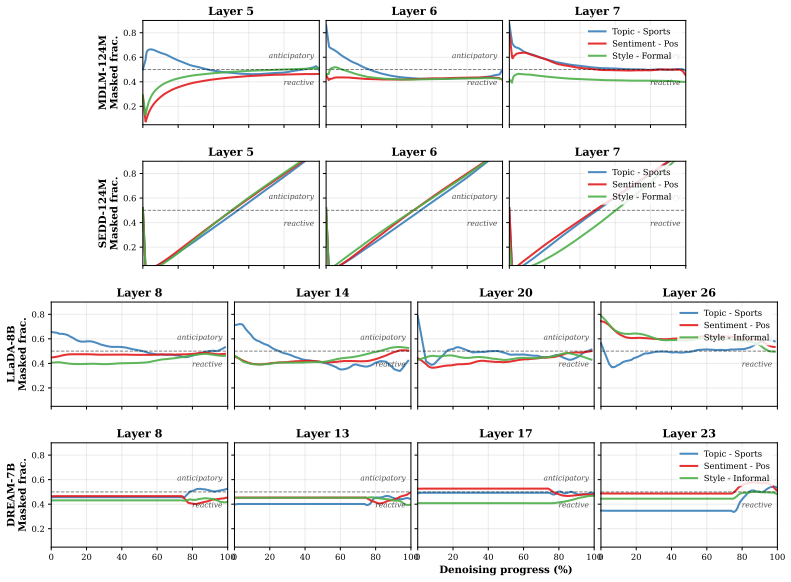
Jacob Austin, Daniel D Johnson, Jonathan Ho, Daniel Tarlow, and Rianne Van Den Berg. Structured denoising diffusion models in discrete state-spaces.Advances in neural information processing systems, 34:17981–17993, 2021
work page 2021
-
[2]
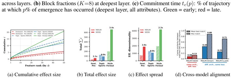
Simple and effective masked diffusion language models
Subham S Sahoo, Marianne Arriola, Yair Schiff, Aaron Gokaslan, Edgar Marroquin, Justin T Chiu, Alexander Rush, and V olodymyr Kuleshov. Simple and effective masked diffusion language models. Advances in Neural Information Processing Systems, 37:130136–130184, 2024
work page 2024
-
[3]
Discrete diffusion modeling by estimating the ratios of the data distribution
Aaron Lou, Chenlin Meng, and Stefano Ermon. Discrete diffusion modeling by estimating the ratios of the data distribution. InInternational Conference on Machine Learning, pages 32819–32848. PMLR, 2024
work page 2024
-
[4]
Dream 7B: Diffusion Large Language Models
Jiacheng Ye, Zhihui Xie, Lin Zheng, Jiahui Gao, Zirui Wu, Xin Jiang, Zhenguo Li, and Lingpeng Kong. Dream 7b: Diffusion large language models.arXiv preprint arXiv:2508.15487, 2025
work page internal anchor Pith review Pith/arXiv arXiv 2025
-
[5]
Large language diffusion models
Shen Nie, Fengqi Zhu, Zebin You, Xiaolu Zhang, Jingyang Ou, Jun Hu, JUN ZHOU, Yankai Lin, Ji-Rong Wen, and Chongxuan Li. Large language diffusion models. InThe Thirty-ninth Annual Conference on Neural Information Processing Systems
-
[6]
Sparse Autoencoders Find Highly Interpretable Features in Language Models
Hoagy Cunningham, Aidan Ewart, Logan Riggs, Robert Huben, and Lee Sharkey. Sparse autoencoders find highly interpretable features in language models.arXiv preprint arXiv:2309.08600, 2023
work page internal anchor Pith review Pith/arXiv arXiv 2023
-
[7]
Trenton Bricken, Adly Templeton, Joshua Batson, Brian Chen, Adam Jermyn, Tom Conerly, et al. Towards monosemanticity: Decomposing language models with dictionary learning.Transformer Circuits Thread, 2023
work page 2023
-
[8]
Adly Templeton, Tom Conerly, Jonathan Marcus, et al. Scaling monosemanticity: Extracting interpretable features from Claude 3 Sonnet.Transformer Circuits Thread, 2024
work page 2024
-
[9]
Breaking bad tokens: Detoxification of llms using sparse autoencoders
Agam Goyal, Vedant Rathi, William Yeh, Yian Wang, Yuen Chen, and Hari Sundaram. Breaking bad tokens: Detoxification of llms using sparse autoencoders. InProceedings of the 2025 Conference on Empirical Methods in Natural Language Processing, pages 12702–12720, 2025
work page 2025
-
[10]
Jehyeok Yeon, Federico Cinus, Yifan Wu, and Luca Luceri. Gsae: Graph-regularized sparse autoencoders for robust llm safety steering.arXiv preprint arXiv:2512.06655, 2025
-
[11]
CorrSteer: Generation-Time LLM Steering via Correlated Sparse Autoencoder Features
Seonglae Cho, Zekun Wu, and Adriano Koshiyama. Corrsteer: Generation-time llm steering via correlated sparse autoencoder features.arXiv preprint arXiv:2508.12535, 2025
work page internal anchor Pith review Pith/arXiv arXiv 2025
-
[12]
SAEs are good for steering – if you select the right features.arXiv preprint arXiv:2505.20063, 2025
Noa Arad, Jonas Mueller, and Yonatan Belinkov. SAEs are good for steering – if you select the right features.arXiv preprint arXiv:2505.20063, 2025. 10
-
[13]
Xu Wang, Bingqing Jiang, Yu Wan, Baosong Yang, Lingpeng Kong, and Difan Zou. Dlm-scope: Mechanis- tic interpretability of diffusion language models via sparse autoencoders.arXiv preprint arXiv:2602.05859, 2026
-
[14]
Eden Avrahami and Eliya Nachmani. Ilrr: Inference-time steering method for masked diffusion language models.arXiv preprint arXiv:2601.21647, 2026
-
[15]
Representation Engineering: A Top-Down Approach to AI Transparency
Andy Zou, Long Phan, Sarah Chen, James Campbell, Phillip Guo, Richard Ren, Alexander Pan, Xuwang Yin, Mantas Mazeika, Ann-Kathrin Dombrowski, et al. Representation engineering: A top-down approach to ai transparency.arXiv preprint arXiv:2310.01405, 2023
work page internal anchor Pith review Pith/arXiv arXiv 2023
-
[16]
Steering llama 2 via contrastive activation addition
Nina Rimsky, Nick Gabrieli, Julian Schulz, Meg Tong, Evan Hubinger, and Alexander Turner. Steering llama 2 via contrastive activation addition. In Lun-Wei Ku, Andre Martins, and Vivek Srikumar, editors, Proceedings of the 62nd Annual Meeting of the Association for Computational Linguistics (Volume 1: Long Papers), pages 15504–15522, Bangkok, Thailand, Aug...
-
[17]
Probing classifiers: Promises, shortcomings, and advances
Yonatan Belinkov. Probing classifiers: Promises, shortcomings, and advances.Computational Linguistics, 48(1):207–219, March 2022. doi: 10.1162/coli_a_00422. URL https://aclanthology.org/2022. cl-1.7/
-
[18]
Narmeen Oozeer, Luke Marks, Fazl Barez, and Amirali Abdullah. Beyond linear steering: Unified multi- attribute control for language models.Findings of the Association for Computational Linguistics: EMNLP, pages 23513–23557, 2025
work page 2025
-
[19]
Or Shafran, Shaked Ronen, Omri Fahn, Shauli Ravfogel, Atticus Geiger, and Mor Geva. From directions to regions: Decomposing activations in language models via local geometry.arXiv preprint arXiv:2602.02464, 2026
-
[20]
Raphael Ronge, Markus Maier, and Frederick Eberhardt. When the coffee feature activates on coffins: An analysis of feature extraction and steering for mechanistic interpretability.arXiv preprint arXiv:2601.03047, 2026
-
[21]
Sanjay Basu, Sadiq Y Patel, Parth Sheth, Bhairavi Muralidharan, Namrata Elamaran, Aakriti Kinra, John Morgan, and Rajaie Batniji. Interpretability without actionability: mechanistic methods cannot correct language model errors despite near-perfect internal representations.arXiv preprint arXiv:2603.18353, 2026
-
[22]
A Comparative analysis of Layer-wise Representational Capacity in AR and Diffusion LLMs
Raghavv Goel, Risheek Garrepalli, Sudhanshu Agrawal, Chris Lott, Mingu Lee, and Fatih Porikli. Skip to the good part: Representation structure & inference-time layer skipping in diffusion vs. autoregressive llms.arXiv preprint arXiv:2603.07475, 2026
work page internal anchor Pith review Pith/arXiv arXiv 2026
-
[23]
Arshia Hemmat, Philip Torr, Yongqiang Chen, and Junchi Yu. Tdgnet: Hallucination detection in diffusion language models via temporal dynamic graphs.arXiv preprint arXiv:2602.08048, 2026
-
[24]
Daniel Son, Sanjana Rathore, Andrew Rufail, Adrian Simon, Daniel Zhang, Soham Dave, Cole Blondin, Kevin Zhu, and Sean O’Brien. Semantic convergence: Investigating shared representations across scaled llms.arXiv preprint arXiv:2507.22918, 2025
-
[25]
Uni- versal sparse autoencoders: Interpretable cross-model concept alignment
Harrish Thasarathan, Julian Forsyth, Thomas Fel, Matthew Kowal, and Konstantinos G Derpanis. Uni- versal sparse autoencoders: Interpretable cross-model concept alignment. InForty-second International Conference on Machine Learning, 2025
work page 2025
-
[26]
Xudong Zhu, Mohammad Mahdi Khalili, and Zhihui Zhu. Abstopk: Rethinking sparse autoencoders for bidirectional features.arXiv preprint arXiv:2510.00404, 2025
-
[27]
Language models are unsupervised multitask learners.OpenAI blog, 1(8):9, 2019
Alec Radford, Jeffrey Wu, Rewon Child, David Luan, Dario Amodei, Ilya Sutskever, et al. Language models are unsupervised multitask learners.OpenAI blog, 1(8):9, 2019
work page 2019
-
[28]
LLaMA: Open and Efficient Foundation Language Models
Hugo Touvron, Thibaut Lavril, Gautier Izacard, Xavier Martinet, Marie-Anne Lachaux, Timothée Lacroix, Baptiste Rozière, Naman Goyal, Eric Hambro, Faisal Azhar, et al. Llama: Open and efficient foundation language models.arXiv preprint arXiv:2302.13971, 2023
work page internal anchor Pith review Pith/arXiv arXiv 2023
-
[29]
An Yang, Baosong Yang, Binyuan Hui, Bo Zheng, Bowen Yu, Chang Zhou, et al. Qwen2 technical report. arXiv preprint arXiv:2407.10671, 2024
work page internal anchor Pith review Pith/arXiv arXiv 2024
-
[30]
Character-level convolutional networks for text classification
Xiang Zhang, Junbo Zhao, and Yann LeCun. Character-level convolutional networks for text classification. Advances in neural information processing systems, 28, 2015. 11
work page 2015
-
[31]
Andrew L. Maas, Raymond E. Daly, Peter T. Pham, Dan Huang, Andrew Y . Ng, and Christopher Potts. Learning word vectors for sentiment analysis. In Dekang Lin, Yuji Matsumoto, and Rada Mihalcea, editors,Proceedings of the 49th Annual Meeting of the Association for Computational Linguistics: Human Language Technologies, pages 142–150, Portland, Oregon, USA, ...
work page 2011
-
[32]
Ellie Pavlick and Joel Tetreault. An empirical analysis of formality in online communication.Transactions of the association for computational linguistics, 4:61–74, 2016
work page 2016
-
[33]
Don’t lose the message while paraphrasing: A study on content preserving style transfer
Nikolay Babakov, David Dale, Ilya Gusev, Irina Krotova, and Alexander Panchenko. Don’t lose the message while paraphrasing: A study on content preserving style transfer. InInternational Conference on Applications of Natural Language to Information Systems, pages 47–61. Springer, 2023
work page 2023
-
[34]
Jacob Cohen.Statistical power analysis for the behavioral sciences. routledge, 2013
work page 2013
-
[35]
Henry B Mann and Donald R Whitney. On a test of whether one of two random variables is stochastically larger than the other.The annals of mathematical statistics, pages 50–60, 1947
work page 1947
-
[36]
Carlo Bonferroni. Teoria statistica delle classi e calcolo delle probabilita.Pubblicazioni del R istituto superiore di scienze economiche e commericiali di firenze, 8:3–62, 1936
work page 1936
-
[37]
Prafulla Dhariwal and Alexander Nichol. Diffusion models beat gans on image synthesis.Advances in neural information processing systems, 34:8780–8794, 2021
work page 2021
-
[38]
DistilBERT, a distilled version of BERT: smaller, faster, cheaper and lighter
Victor Sanh, Lysandre Debut, Julien Chaumond, and Thomas Wolf. Distilbert, a distilled version of bert: smaller, faster, cheaper and lighter.arXiv preprint arXiv:1910.01108, 2019
work page internal anchor Pith review Pith/arXiv arXiv 1910
-
[39]
Bert: Pre-training of deep bidi- rectional transformers for language understanding
Jacob Devlin, Ming-Wei Chang, Kenton Lee, and Kristina Toutanova. Bert: Pre-training of deep bidi- rectional transformers for language understanding. InProceedings of the 2019 conference of the North American chapter of the association for computational linguistics: human language technologies, volume 1 (long and short papers), pages 4171–4186, 2019
work page 2019
-
[40]
David L Donoho and Michael Elad. Optimally sparse representation in general (nonorthogonal) dictionaries via l1 minimization.Proceedings of the National Academy of Sciences, 100(5):2197–2202, 2003
work page 2003
-
[41]
Alireza Makhzani and Brendan Frey. K-sparse autoencoders.arXiv preprint arXiv:1312.5663, 2013
-
[42]
Eliciting Latent Predictions from Transformers with the Tuned Lens
Nora Belrose, Igor Ostrovsky, Lev McKinney, Zach Furman, Logan Smith, Danny Halawi, Stella Biderman, and Jacob Steinhardt. Eliciting latent predictions from transformers with the tuned lens.arXiv preprint arXiv:2303.08112, 2023
work page internal anchor Pith review Pith/arXiv arXiv 2023
- [43]
-
[44]
Cambridge University Press, 2015
Jordan J Louviere, Terry N Flynn, and Anthony Alfred John Marley.Best-worst scaling: Theory, methods and applications. Cambridge University Press, 2015
work page 2015
-
[45]
Sudha Rao and Joel Tetreault. Dear sir or madam, may i introduce the gyafc dataset: Corpus, benchmarks and metrics for formality style transfer. InProceedings of the 2018 conference of the north american chapter of the association for computational linguistics: human language technologies, volume 1 (long papers), pages 129–140, 2018
work page 2018
-
[46]
Barry Payne Welford. Note on a method for calculating corrected sums of squares and products.Techno- metrics, 4(3):419–420, 1962. 12 A Proofs and Extended Discussion for Steering Methods We restate each result for convenience and provide full proofs. A.1 Proof of Theorem 1 (Adaptive-vs-uniform efficiency ratio) A.1.1 Trajectory-level KL: exact additive de...
work page 1962
-
[47]
We probe two attributes: sentiment (IMDB, 2- class) and topic (AG News, 4-class)
Linear probing.Logistic regression with 5-fold stratified cross-validation on mean-pooled activations from every transformer layer. We probe two attributes: sentiment (IMDB, 2- class) and topic (AG News, 4-class). To account for the stochastic nature of diffusion representations, each text is passed through the model with 3 independent noise samples (mask...
-
[48]
We monitor reconstruction loss and dead neuron fraction as quality indicators
SAE training.TopK SAEs are trained on candidate layers with identical hyperparameters per model (Table 10), ensuring fair comparison. We monitor reconstruction loss and dead neuron fraction as quality indicators
-
[49]
This reveals which layers produce the strongest and most numerous attribute-discriminative features
Contrastive feature identification.Per-feature Cohen’s d between attribute groups, retain- ing features with |d|>0.05 and p <0.01 . This reveals which layers produce the strongest and most numerous attribute-discriminative features
-
[50]
Steering ablation.The decisive test: we compare steering effectiveness (positive-rate swing across an α sweep) for different layer windows, isolating the causal contribution of each layer group. C.3.2 Layer Probing Results Table 8 reports sentiment probing accuracy at selected layers for all four models. Three patterns emerge: 25 Table 8: Linear probing a...
-
[51]
SEDD (score- entropy loss) shows no dissociation — later layers both probe and steer best
Probing–steering dissociation is loss-dependent.MDLM (absorbing loss) shows clear dissociation — middle layers steer best despite later layers probing best. SEDD (score- entropy loss) shows no dissociation — later layers both probe and steer best. LLaDA shows suggestive dissociation similar to MDLM. This implicates the training objective, not the architec...
-
[52]
The causal malleability principle extends to diffusion transformers.For absorbing-loss DLMs, middle layers provide the best balance of representational richness and propagation distance, consistent with findings from autoregressive representation engineering. This principle appears robust across model scales (124M to 8B) and architectures (GPT-2, Qwen2, L...
-
[53]
Tokenization:We tokenize each text with the model’s tokenizer, truncating or padding to the model’s sequence length. 2.Apply noise:Then for each text, we create 3 noised versions at mask ratios{0.3,0.5,0.7} by randomly replacing tokens with [MASK]. This ensures features are identified across noise levels rather than at a single denoising stage
-
[54]
Forward pass:Next, we run the noised input through the model to obtain hidden states at each SAE layer
-
[55]
ReLU SAE encoding (per-token):for each token position at each SAE layer, we compute: activations= ReLU (h−b dec)W enc +b enc ,(15) This produces a (seq_len×d SAE) activation matrix per sample per layer. Although the SAEs use TopK activation during training and normal inference, we use full ReLU encoding for 1https://huggingface.co/s-nlp/roberta-base-forma...
-
[56]
Streaming statistics:We accumulate per-feature mean and variance for class A and class B using Welford’s online algorithm [46], avoiding the need to store all activations in memory. 6.Cohen’sd[34]:for each of thed SAE features at each layer, we compute: dj = ¯hA j − ¯hB jq (Var(hA j ) + Var(hB j ))/2 .(16) Positivedindicates a feature more active for clas...
-
[57]
Statistical validation:Next, we rank features by |d|, take the top 300 candidates, and run Mann-Whitney U tests [35] with p <0.01 (Bonferroni-corrected [36] across 300 tests). We retain the top 50 positive-d and top 50 negative-d features per layer (indices and statistics) for our study. The top 20 per direction are used for steering. 8.Per-feature mean s...
-
[58]
We generateNsamples with SAE hooks active at all denoising steps
-
[59]
At each step, we ReLU-encode the hidden states through the SAE and record activations for the top-20 contrastive features per attribute
-
[60]
We store per-sample, per-step activations as an(N×T×F) tensor per layer, where T is the number of denoising steps andFis the number of tracked features. 31
-
[61]
Since not all generated samples express the target attribute, we classify all N texts with attribute-specific classifiers (Table 16) and retain only confident samples (softmax probability above a threshold; see Table 17) to avoid diluting the emergence signal. Informality uses a lower threshold (0.6) because baseline formality is high (81–85% for LLaDA/DR...
-
[62]
Then we average dynamics over the filtered samples to obtain per-step mean activation curves
-
[63]
We compute block fractions by dividing the trajectory into B temporal blocks, computing the activation change in each block, clamping negatives to zero, and normalizing to sum to one. Table 16: Evaluation classifiers. These classifiers are used for evaluation and for filtering dynamics samples. They are not used during contrastive feature extraction for s...
-
[64]
We generate N samples (Table 18) with SAE hooks active at every denoising step, recording per-step activations for the top-20 contrastive features per attribute per layer
-
[65]
We filter to classifier-confident samples (Table 17) and average across retained samples to obtain a per-step mean activation curve ¯h(t)
-
[66]
We compute absolute deviation from baseline: |¯h(t)− ¯h(0)|, which captures emergence regardless of whether the mean activation increases or decreases during denoising
-
[67]
We apply moving-average smoothing with model-specific window sizes (MDLM/SEDD: no smoothing for 1024-step trajectories since they are sufficiently smooth; LLaDA: window= 5 for 64-step trajectories; DREAM: window = 9 for 256-step trajectories) to reduce per-step noise while preserving emergence timing
-
[68]
Each panel in Figure 6 shows a single model–attribute combination, with one line per SAE layer
We normalize each curve to [0,1] via min-max scaling, so that 0 corresponds to baseline (fully masked) and1to full emergence. Each panel in Figure 6 shows a single model–attribute combination, with one line per SAE layer. This reveals both thetimingof emergence (how early or late features activate) and thedepth gradient (whether shallow or deep layers com...
-
[69]
The denoising trajectory is divided into K=8 equal temporal blocks. For MDLM/SEDD (1024 steps), each block spans 128 steps; for LLaDA (64 steps), 8 steps; for DREAM (256 steps), 32 steps
-
[70]
For each block b, we compute the activation increase from the block’s start to its end: δb = ¯h(eb)− ¯h(sb), wheres b ande b are the first and last steps of blockb
-
[71]
Negative deltas are clamped to zero: δ+ b = max(0, δ b). This prevents blocks where activation temporarily decreases (e.g., due to non-monotonic trajectories) from receiving negative weight
-
[72]
Block fractions are computed by normalizing:f b =δ + b /P b′ δ+ b′ , so they sum to one. Figure 7 presents the full results, organized as a 4-row grid (one row per model, one column per layer). The deepest-layer panels correspond to the main paper’s Figure 2b. 36 B0 B2 B4 B6 Denoising block 0% 20% 40% 60% 80% 100% MDLM-124M % of emergence Layer 5 Sentimen...
-
[73]
We load the full set of dSAE Cohen’sd values computed during contrastive feature extraction (§C.5.2)
-
[74]
We take the absolute value|d j|and sort features in descending order
-
[75]
We plot the cumulative sumPr i=1 |d(i)|versus feature rankrfor the top 50 features. The cumulative |d| curve captures how discriminative signal is distributed across features: a steep initial rise indicates that a few features carry most of the signal (concentrated representation), while a gradual rise indicates distributed encoding across many features. ...
work page 2011
discussion (0)
Sign in with ORCID, Apple, or X to comment. Anyone can read and Pith papers without signing in.