Understanding Deterioration Random Effects for Causal Discovery in Infrastructure Management
Pith reviewed 2026-05-21 06:59 UTC · model grok-4.3
The pith
Stratifying Bayesian random effects by sign uncovers that low-risk pumps have 400 times stronger causal drivers of deterioration than high-risk ones.
A machine-rendered reading of the paper's core claim, the machinery that carries it, and where it could break.
Core claim
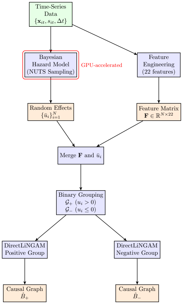
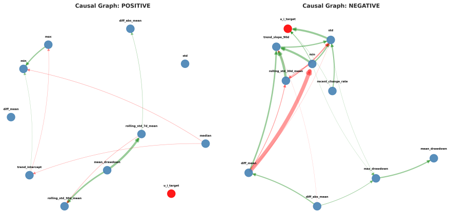
The central claim is that estimating pump-specific random effects u_i via GPU-accelerated NUTS sampling in a hierarchical hazard model, followed by DirectLiNGAM causal discovery stratified on the sign of those effects, reveals that the negative random-effects group exhibits causal effects 400 times larger than the positive group, with the standard deviation feature showing a strong positive causal effect of +1.515 on deterioration rates specifically in the low-risk equipment.
What carries the argument
Stratification of DirectLiNGAM causal discovery by the sign of Bayesian-estimated random effects u_i, which separates faster-deteriorating and slower-deteriorating regimes for independent feature-to-rate causal graphs.
If this is right
- Maintenance strategies must be tailored separately to the operational patterns that dominate in low-risk versus high-risk equipment.
- Standard deviation of time-series measurements becomes a high-leverage monitoring target for the slower-deterioration subgroup.
- GPU acceleration makes the combined Bayesian sampling and causal discovery workflow practical for large sensor datasets.
- NonlinearLiNGAM checks confirm that the linear causal assumptions hold sufficiently for the reported effect sizes.
Where Pith is reading between the lines
- The same stratification idea could be tested on other infrastructure assets such as bridges or pipelines to check whether random-effect sign consistently isolates distinct causal regimes.
- Iterating between random-effect estimation and causal discovery in a joint loop might reduce any residual dependence between the grouping step and the discovered graphs.
- Real-time systems could monitor incoming data streams to re-assign a pump to the positive or negative regime and switch the active causal model accordingly.
Load-bearing premise
Dividing the data by the sign of the fitted random effects u_i produces causally valid subgroups without selection bias or confounding introduced by the estimation step itself.
What would settle it
Re-estimating the random effects after an initial sign-based split and finding that the 400-fold difference in causal effect magnitudes largely disappears would falsify the claim that the stratification isolates distinct causal regimes.
Figures


read the original abstract
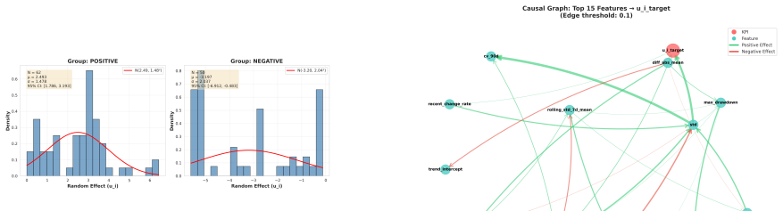
Infrastructure deterioration poses significant challenges for asset management, yet existing approaches rely on population-averaged models that overlook equipment-specific heterogeneity. We present a novel framework that combines Bayesian hierarchical hazard modeling with causal discovery to identify operational patterns that drive heterogeneous deterioration rates in pump equipment. Our approach first estimates pump-specific random effects $u_i$ using GPU-accelerated No-U-Turn Sampling (NUTS), achieving 3--5$\times$ speedup over CPU implementations. We then employ DirectLiNGAM to discover causal relationships between 22 engineered time-series features and deterioration rates, stratified by positive ($u_i > 0$, faster deterioration) versus negative ($u_i \leq 0$, slower deterioration) random effects. Analyzing 112 pumps with 92,861 observations over 650 days, we uncover striking heterogeneity: the negative group exhibits causal effects 400$\times$ larger than the positive group, with standard deviation (std) showing a strong positive causal effect ($+1.515$) on deterioration rates in low-risk equipment. We validate linearity assumptions through NonlinearLiNGAM comparison and demonstrate practical scalability through GPU acceleration. Our findings enable targeted maintenance strategies by revealing that different operational regimes require fundamentally distinct management approaches, advancing predictive maintenance from population-averaged to heterogeneity-aware decision making.
Editorial analysis
A structured set of objections, weighed in public.
Referee Report
Summary. The manuscript proposes a framework that first fits a Bayesian hierarchical hazard model to estimate pump-specific random effects u_i via GPU-accelerated NUTS sampling on deterioration trajectories, then stratifies the 112 pumps into positive (u_i > 0) and negative (u_i ≤ 0) groups and applies DirectLiNGAM to discover causal effects of 22 engineered time-series features on deterioration rates within each stratum. The central empirical claim is that the negative group shows causal effects approximately 400 times larger than the positive group, including a strong positive effect of +1.515 for the standard-deviation feature in low-risk equipment, with linearity validated by comparison to NonlinearLiNGAM.
Significance. If the stratification step can be shown to be free of selection bias, the demonstration of strong heterogeneity in causal drivers would support moving from population-averaged to subgroup-specific maintenance policies in infrastructure management. The GPU acceleration and explicit linearity check are concrete methodological strengths that improve reproducibility of the computational pipeline.
major comments (1)
- [Abstract] Abstract (stratified causal discovery paragraph): the reported 400× difference in causal effect magnitudes and the +1.515 coefficient on std in the negative group are obtained after stratifying on the sign of the fitted random effects u_i. Because these u_i are posterior estimates derived from the same pump-level deterioration observations that later serve as the outcome variable in DirectLiNGAM, the stratification is a post-selection operation on a noisy function of the target. This mechanism can induce spurious within-stratum associations even in the absence of true causal heterogeneity; the manuscript provides no diagnostic (permutation test of the grouping, comparison against pre-estimation clustering, or sensitivity to u_i uncertainty) that would rule out this artifact.
minor comments (2)
- The abstract does not specify the exact functional form of the hazard model (e.g., baseline hazard, link function, or how the random effect enters the linear predictor) or the precise definitions and preprocessing steps for the 22 engineered time-series features.
- No discussion is given of how posterior uncertainty in the estimated u_i propagates into the subsequent LiNGAM coefficient estimates or into the reported 400× ratio.
Simulated Author's Rebuttal
We thank the referee for their detailed and constructive review. We value the recognition of the framework's methodological strengths and the importance of the heterogeneity findings. We address the major comment on potential selection bias in the stratification below, proposing concrete revisions to strengthen the analysis.
read point-by-point responses
-
Referee: [Abstract] Abstract (stratified causal discovery paragraph): the reported 400× difference in causal effect magnitudes and the +1.515 coefficient on std in the negative group are obtained after stratifying on the sign of the fitted random effects u_i. Because these u_i are posterior estimates derived from the same pump-level deterioration observations that later serve as the outcome variable in DirectLiNGAM, the stratification is a post-selection operation on a noisy function of the target. This mechanism can induce spurious within-stratum associations even in the absence of true causal heterogeneity; the manuscript provides no diagnostic (permutation test of the grouping, comparison against pre-estimation clustering, or sensitivity to u_i uncertainty) that would rule out this artifact.
Authors: We thank the referee for identifying this important methodological consideration. The random effects u_i are indeed posterior estimates from the hierarchical hazard model applied to the deterioration trajectories, and the subsequent stratification on their sign followed by DirectLiNGAM on deterioration rates as the target could introduce dependence. While the u_i capture pump-specific baseline deviations and the causal discovery focuses on feature-driven variations within strata, we acknowledge that this post-selection step warrants explicit validation to rule out artifacts. In the revision, we will add a dedicated robustness subsection that includes: (1) a permutation test that randomly reassigns pumps to strata (preserving group sizes) and recomputes the causal effect magnitudes to assess whether the observed 400× difference exceeds what arises under random grouping; (2) a sensitivity analysis that draws multiple samples from the posterior distribution of u_i, re-stratifies, and reports variability in the DirectLiNGAM coefficients; and (3) a comparison of results against an alternative pre-estimation clustering approach based solely on raw deterioration statistics. These diagnostics will be reported with quantitative results and will directly address the concern of spurious associations. revision: yes
Circularity Check
Stratification by sign of fitted random effects u_i creates dependence between grouping and deterioration outcome
specific steps
-
fitted input called prediction
[Abstract (stratified causal discovery paragraph)]
"We then employ DirectLiNGAM to discover causal relationships between 22 engineered time-series features and deterioration rates, stratified by positive ($u_i > 0$, faster deterioration) versus negative ($u_i ≤ 0$, slower deterioration) random effects."
u_i is obtained by NUTS sampling from the hierarchical model whose likelihood is the observed deterioration trajectories; sign(u_i) is therefore a direct function of the same outcome variable later used as the LiNGAM target. Conditioning the causal analysis on this fitted quantity makes the reported within-stratum coefficients (including the 400× difference and +1.515 on std) statistically dependent on the estimation step rather than arising from an independent discovery process.
full rationale
The derivation proceeds by first fitting pump-specific random effects u_i via Bayesian hierarchical hazard model on the deterioration trajectories, then stratifying the identical observations by sign(u_i) before running DirectLiNGAM on features versus deterioration rates. This step is load-bearing for the headline claim of 400× heterogeneity and the +1.515 coefficient; the strata are defined directly from a posterior function of the target variable, inducing statistical dependence that is not independently validated. No self-citation chain or ansatz smuggling is present, but the fitted-input conditioning reduces the causal-discovery results to a post-selection analysis of the same data.
Axiom & Free-Parameter Ledger
free parameters (1)
- pump-specific random effects u_i
axioms (2)
- domain assumption Linearity assumption for causal effects in DirectLiNGAM
- domain assumption Hazard function form and prior distributions in the Bayesian model
Lean theorems connected to this paper
-
IndisputableMonolith/Foundation/AbsoluteFloorClosure.leanabsolute_floor_iff_bare_distinguishability unclear?
unclearRelation between the paper passage and the cited Recognition theorem.
We then employ DirectLiNGAM to discover causal relationships between 22 engineered time-series features and deterioration rates, stratified by positive (u_i > 0, faster deterioration) versus negative (u_i ≤ 0, slower deterioration) random effects.
-
IndisputableMonolith/Cost/FunctionalEquation.leanwashburn_uniqueness_aczel unclear?
unclearRelation between the paper passage and the cited Recognition theorem.
the negative group exhibits causal effects 400× larger than the positive group, with standard deviation (std) showing a strong positive causal effect (+1.515)
What do these tags mean?
- matches
- The paper's claim is directly supported by a theorem in the formal canon.
- supports
- The theorem supports part of the paper's argument, but the paper may add assumptions or extra steps.
- extends
- The paper goes beyond the formal theorem; the theorem is a base layer rather than the whole result.
- uses
- The paper appears to rely on the theorem as machinery.
- contradicts
- The paper's claim conflicts with a theorem or certificate in the canon.
- unclear
- Pith found a possible connection, but the passage is too broad, indirect, or ambiguous to say the theorem truly supports the claim.
Reference graph
Works this paper leans on
-
[1]
Estimation of infrastructure transition probabilities from condition rating data,
S. M. Madanat, W. B. Mishalani, and W. H. Ibrahim, “Estimation of infrastructure transition probabilities from condition rating data,”Jour- nal of Infrastructure Systems, vol. 1, no. 2, pp. 120–125, 1995
work page 1995
-
[2]
Estimation in generalized linear mod- els with random effects,
R. Schall, “Estimation in generalized linear mod- els with random effects,”Biometrika, vol. 78, no. 4, pp. 719–727, 1991
work page 1991
-
[3]
P. Spirtes, C. Glymour, and R. Scheines,Causa- tion, Prediction, and Search, 2nd ed. MIT Press, 2000
work page 2000
-
[4]
Pearl,Causality: Models, Reasoning, and Inference, 2nd ed
J. Pearl,Causality: Models, Reasoning, and Inference, 2nd ed. Cambridge University Press, 2009
work page 2009
-
[5]
A linear non-Gaussian acyclic model for causal discovery,
S. Shimizu, P. O. Hoyer, A. Hyv¨ arinen, and A. Kerminen, “A linear non-Gaussian acyclic model for causal discovery,”Journal of Machine Learning Research, vol. 7, pp. 2003–2030, 2006
work page 2003
-
[6]
The No-U- Turn Sampler: Adaptively setting path lengths in Hamiltonian Monte Carlo,
M. D. Hoffman and A. Gelman, “The No-U- Turn Sampler: Adaptively setting path lengths in Hamiltonian Monte Carlo,”Journal of Ma- chine Learning Research, vol. 15, pp. 1593–1623, 2014
work page 2014
-
[7]
Hamiltonian Monte Carlo for hierarchical models,
M. Betancourt and M. Girolami, “Hamiltonian Monte Carlo for hierarchical models,”Current Trends in Bayesian Methodology with Applica- tions, pp. 79–101, 2015
work page 2015
-
[8]
DirectLiNGAM: A direct method for learning a linear non-Gaussian structural equation model,
S. Shimizu, T. Inazumi, Y. Sogawa, A. Hyv¨ arinen, Y. Kawahara, T. Washio, P. O. Hoyer, and K. Bollen, “DirectLiNGAM: A direct method for learning a linear non-Gaussian structural equation model,”Journal of Machine Learning Research, vol. 12, pp. 1225–1248, 2011
work page 2011
-
[9]
Regression models and life-tables,
D. R. Cox, “Regression models and life-tables,” Journal of the Royal Statistical Society: Series B, vol. 34, no. 2, pp. 187–220, 1972
work page 1972
- [10]
-
[11]
FedAvg-Based CTMC Hazard Model for Federated Bridge Deterioration As- sessment,
T. Yasuno, “FedAvg-Based CTMC Hazard Model for Federated Bridge Deterioration As- sessment,”arXiv preprint arXiv:2602.20194, 2026
-
[12]
T. Yasuno, M. Okano, and J. Fujii, “Wooden sleeper deterioration detection for rural railway prognostics using unsupervised deeper FCDDs,” arXiv preprint arXiv:2305.05103, 2023
-
[13]
L. Breiman, “Random forests,”Machine Learn- ing, vol. 45, no. 1, pp. 5–32, 2001
work page 2001
-
[14]
Greedy function approxima- tion: A gradient boosting machine,
J. H. Friedman, “Greedy function approxima- tion: A gradient boosting machine,”Annals of Statistics, vol. 29, no. 5, pp. 1189–1232, 2001
work page 2001
-
[15]
W. Zhang, C. Li, G. Peng, Y. Chen, and Z. Zhang, “A deep convolutional neural network with new training methods for bearing fault di- agnosis under noisy environment and different working load,”Mechanical Systems and Signal Processing, vol. 100, pp. 439–453, 2018
work page 2018
-
[16]
A unified ap- proach to interpreting model predictions,
S. M. Lundberg and S.-I. Lee, “A unified ap- proach to interpreting model predictions,” in Advances in Neural Information Processing Sys- tems, vol. 30, 2017
work page 2017
-
[17]
T. Yasuno, M. Okano, and J. Fujii, “One- class Damage Detector Using Deeper Fully- Convolutional Data Descriptions for Civil Appli- cation,”arXiv preprint arXiv:2303.01732, 2023
-
[18]
T. Yasuno, “Hybrid Feature Learning with Time Series Embeddings for Equipment Anomaly Pre- diction,”arXiv preprint arXiv:2602.15089, 2026
work page internal anchor Pith review Pith/arXiv arXiv 2026
-
[19]
Causal inference in the presence of latent variables and selection bias,
P. Spirtes, C. Meek, and T. Richardson, “Causal inference in the presence of latent variables and selection bias,” inProceedings of the Eleventh Conference on Uncertainty in Artificial Intelli- gence, pp. 499–506, 1995
work page 1995
-
[20]
Optimal structure identifi- cation with greedy search,
D. M. Chickering, “Optimal structure identifi- cation with greedy search,”Journal of Machine Learning Research, vol. 3, pp. 507–554, 2002
work page 2002
-
[21]
Learning Bayesian networks: The combina- tion of knowledge and statistical data,
D. Heckerman, D. Geiger, and D. M. Chicker- ing, “Learning Bayesian networks: The combina- tion of knowledge and statistical data,”Machine Learning, vol. 20, no. 3, pp. 197–243, 1995. 16
work page 1995
-
[22]
Nonlinear causal discovery with additive noise models,
P. O. Hoyer, D. Janzing, J. M. Mooij, J. Peters, and B. Sch¨ olkopf, “Nonlinear causal discovery with additive noise models,”Advances in Neural Information Processing Systems, vol. 21, 2008
work page 2008
-
[23]
Estimation of a structural vector autore- gression model using non-Gaussianity,
A. Hyv¨ arinen, K. Zhang, S. Shimizu, and P. O. Hoyer, “Estimation of a structural vector autore- gression model using non-Gaussianity,”Journal of Machine Learning Research, vol. 11, pp. 1709– 1731, 2010
work page 2010
-
[24]
Investigating causal relations by econometric models and cross-spectral meth- ods,
C. W. Granger, “Investigating causal relations by econometric models and cross-spectral meth- ods,”Econometrica, vol. 37, no. 3, pp. 424–438, 1969
work page 1969
-
[25]
Dynamic Bayesian networks: Representation, inference and learning,
K. P. Murphy, “Dynamic Bayesian networks: Representation, inference and learning,” PhD thesis, UC Berkeley, 2002
work page 2002
-
[26]
High-recall causal discovery for autocorrelated time series with la- tent confounders,
A. Gerhardus and J. Runge, “High-recall causal discovery for autocorrelated time series with la- tent confounders,”Advances in Neural Infor- mation Processing Systems, vol. 33, pp. 12615– 12625, 2020
work page 2020
- [27]
-
[28]
A note on modeling vehicle accident frequencies with random-parameters count models,
P. C. Anastasopoulos and F. L. Mannering, “A note on modeling vehicle accident frequencies with random-parameters count models,”Acci- dent Analysis & Prevention, vol. 41, no. 1, pp. 153–159, 2009
work page 2009
-
[29]
L. Gao and Z. Zhang, “Robust multivariate and functional archetypal analysis with application to financial time series analysis,”Physica A: Sta- tistical Mechanics and its Applications, vol. 391, no. 3, pp. 811–822, 2012
work page 2012
-
[30]
Stochastic relaxation, Gibbs distributions, and the Bayesian restora- tion of images,
S. Geman and D. Geman, “Stochastic relaxation, Gibbs distributions, and the Bayesian restora- tion of images,”IEEE Transactions on Pattern Analysis and Machine Intelligence, vol. PAMI-6, no. 6, pp. 721–741, 1984
work page 1984
-
[31]
Monte Carlo sampling meth- ods using Markov chains and their applications,
W. K. Hastings, “Monte Carlo sampling meth- ods using Markov chains and their applications,” Biometrika, vol. 57, no. 1, pp. 97–109, 1970
work page 1970
-
[32]
MCMC using Hamiltonian dynam- ics,
R. M. Neal, “MCMC using Hamiltonian dynam- ics,” inHandbook of Markov Chain Monte Carlo (S. Brooks et al., eds.), pp. 113–162, CRC Press, 2011
work page 2011
-
[33]
Probabilistic programming in Python us- ing PyMC3,
J. Salvatier, T. V. Wiecki, and C. Fonnes- beck, “Probabilistic programming in Python us- ing PyMC3,”PeerJ Computer Science, vol. 2, p. e55, 2016
work page 2016
-
[34]
Stan: A probabilistic programming language,
B. Carpenter, A. Gelman, M. D. Hoff- man, D. Lee, B. Goodrich, M. Betancourt, M. Brubaker, J. Guo, P. Li, and A. Riddell, “Stan: A probabilistic programming language,” Journal of Statistical Software, vol. 76, no. 1, 2017
work page 2017
-
[35]
Composable Effects for Flexible and Accelerated Probabilistic Programming in NumPyro
D. Phan, N. Pradhan, and M. Jankowiak, “Com- posable effects for flexible and accelerated prob- abilistic programming in NumPyro,”arXiv preprint arXiv:1912.11554, 2019
work page internal anchor Pith review Pith/arXiv arXiv 1912
-
[36]
JAX: Composable transfor- mations of Python+NumPy programs,
J. Bradbury, R. Frostig, P. Hawkins, M. J. Johnson, C. Leary, D. Maclaurin, G. Necula, A. Paszke, J. VanderPlas, S. Wanderman-Milne, and Q. Zhang, “JAX: Composable transfor- mations of Python+NumPy programs,”http: //github.com/google/jax, 2018
work page 2018
-
[37]
Estimation and in- ference of heterogeneous treatment effects using random forests,
S. Wager and S. Athey, “Estimation and in- ference of heterogeneous treatment effects using random forests,”Journal of the American Sta- tistical Association, vol. 113, no. 523, pp. 1228– 1242, 2018
work page 2018
-
[38]
DAGs with NO TEARS: Contin- uous optimization for structure learning,
X. Zheng, B. Aragam, P. K. Ravikumar, and E. P. Xing, “DAGs with NO TEARS: Contin- uous optimization for structure learning,”Ad- vances in Neural Information Processing Sys- tems, vol. 31, 2018
work page 2018
-
[39]
A discovery algorithm for di- rected cyclic graphs,
T. Richardson, “A discovery algorithm for di- rected cyclic graphs,” inProceedings of the Twelfth Conference on Uncertainty in Artificial Intelligence, pp. 454–461, 1996
work page 1996
-
[40]
Sensitivity analysis without assumptions,
P. Ding and T. J. VanderWeele, “Sensitivity analysis without assumptions,”Epidemiology, vol. 27, no. 3, pp. 368–377, 2016
work page 2016
-
[41]
On Markov chain Monte Carlo methods for tall data,
R. Bardenet, A. Doucet, and C. Holmes, “On Markov chain Monte Carlo methods for tall data,”Journal of Machine Learning Research, vol. 18, no. 1, pp. 1515–1557, 2017
work page 2017
-
[42]
Deep fea- ture synthesis: Towards automating data science endeavors,
J. M. Kanter and K. Veeramachaneni, “Deep fea- ture synthesis: Towards automating data science endeavors,” in2015 IEEE International Confer- ence on Data Science and Advanced Analytics, pp. 1–10, 2015. 17 Time-Series Data {xit, sit,∆t} Bayesian Hazard Model (NUTS Sampling) Random Effects {¯ui}N i=1 Feature Engineering (22 features) Feature Matrix F∈R N×22...
work page 2015
discussion (0)
Sign in with ORCID, Apple, or X to comment. Anyone can read and Pith papers without signing in.