Solve for the Hyperparameter, Skip the Search: Kolmogorov-Optimal Scaling Laws for Spline Regression
Pith reviewed 2026-06-26 08:49 UTC · model grok-4.3
The pith
Spline regression optimal resolution follows from a closed-form expression using Kolmogorov widths and a single-fit error estimate rather than grid search.
A machine-rendered reading of the paper's core claim, the machinery that carries it, and where it could break.
Core claim
The optimal resolution G* is the analytic minimizer obtained by setting the derivative of estimated risk (Kolmogorov-powered bias plus PRESS-derived variance) to zero; when the input is replaced by interaction order r in the ANOVA decomposition the same minimizer yields power-law scaling of both optimal G and risk with effective density n divided by the number of active r-way terms, independent of ambient dimension d.
What carries the argument
The Kolmogorov n-width of the smoothness class, which supplies the exact power-law form of squared bias as a function of resolution G.
If this is right
- Optimal resolution and risk become explicit power functions of sample size per active interaction component.
- Ambient input dimension drops out of the exponent once interaction order is fixed.
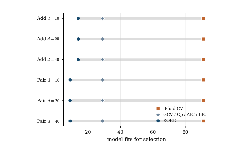
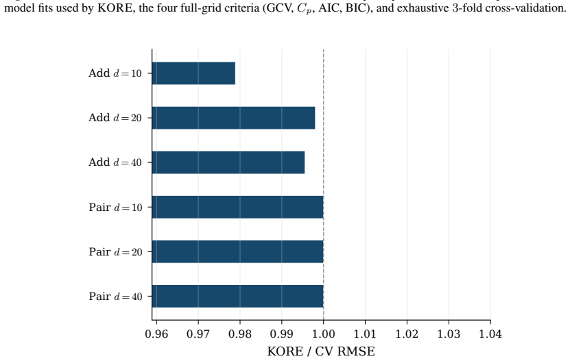
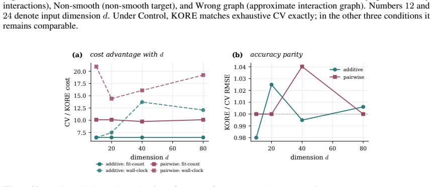
- KORE performs roughly eight times fewer fits than a full grid sweep while matching exhaustive 3-fold cross-validation.
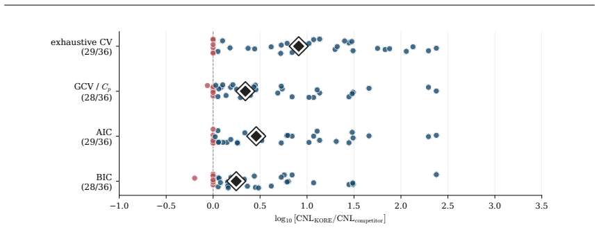
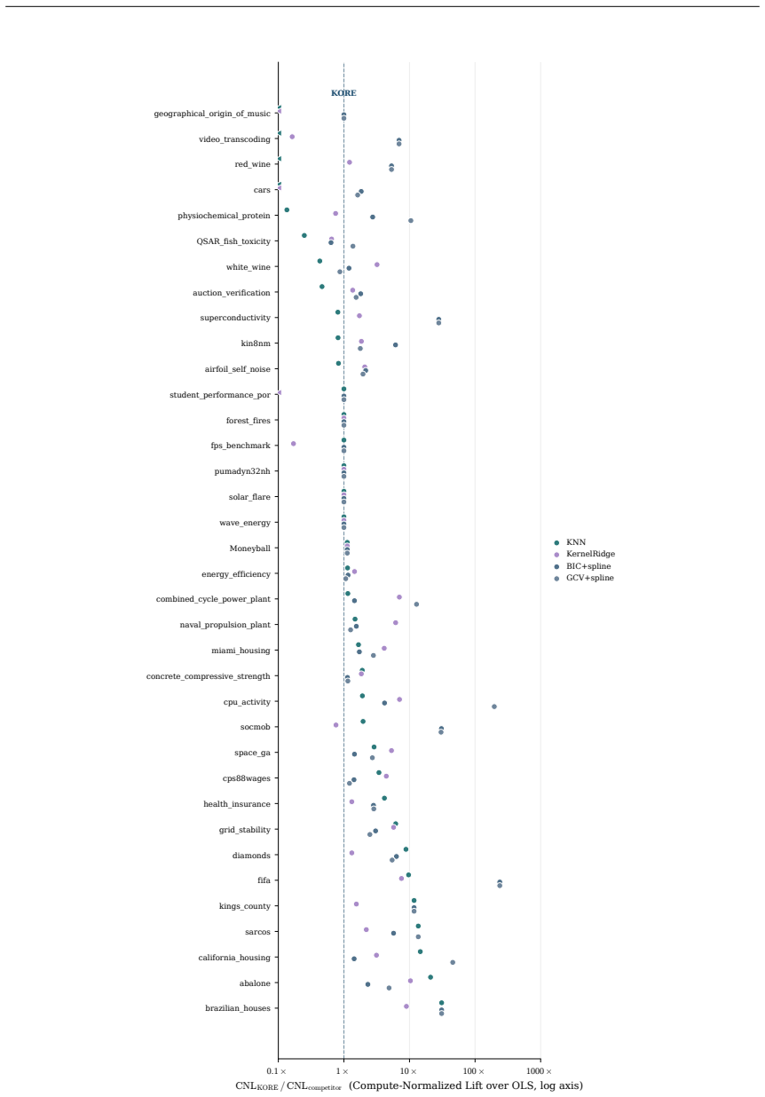
- On tabular data the method ranks first among twenty-one competitors in accuracy per unit compute.
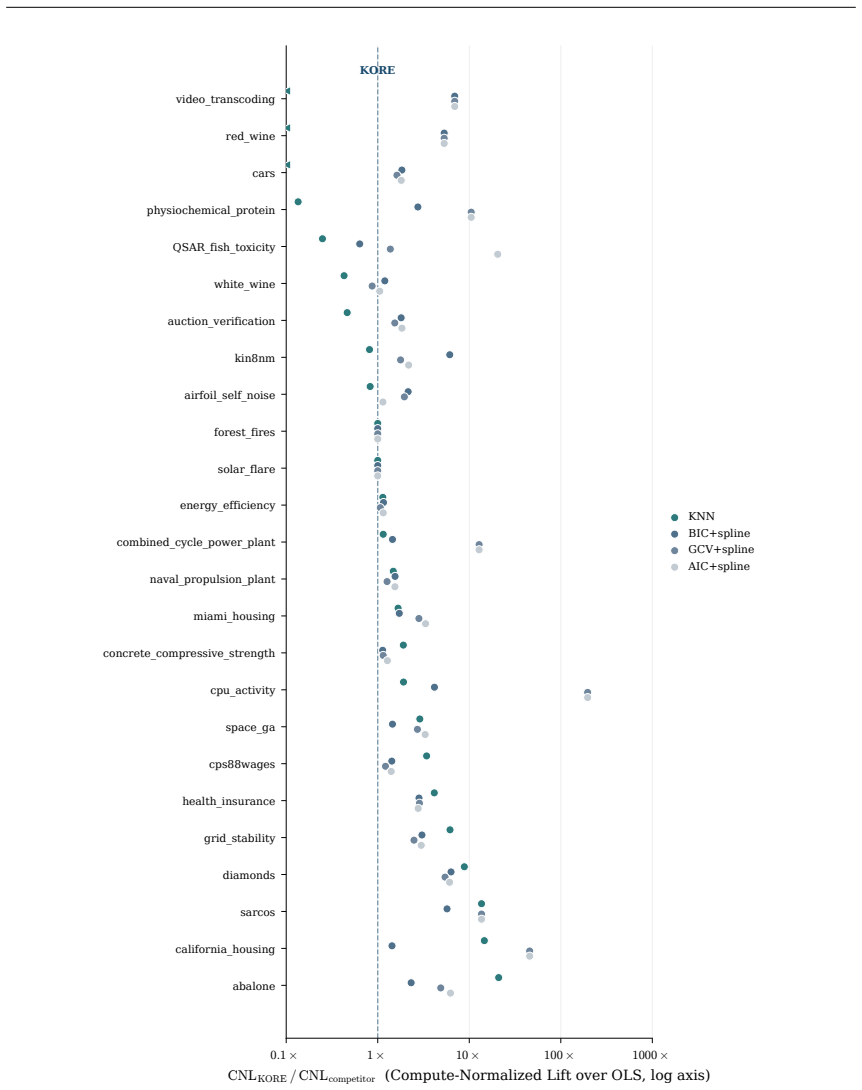
- The same analytic balance reproduces the ordering produced by GCV, Mallows Cp, AIC and BIC.
Where Pith is reading between the lines
- If approximation rates are known for other bases, the same two-pilot calibration could replace search for their resolution or bandwidth parameters.
- The interaction-order reduction suggests that problems whose complexity lives in low-order terms remain tractable even when ambient dimension grows.
- The leave-one-out certificate after the closed-form evaluation supplies a cheap consistency check that could be used to decide whether a third pilot fit is warranted.
Load-bearing premise
Squared bias equals exactly a known power of resolution G given by the Kolmogorov n-width of the smoothness class.
What would settle it
On data drawn from a function whose smoothness class is known in advance, compare the closed-form resolution against the resolution that actually minimizes out-of-sample error; a large systematic difference falsifies the claim.
Figures


read the original abstract
Hyperparameter tuning almost always means search: fit the model at every value on a grid, score each by cross-validation, and keep the winner. For spline regression that search is unnecessary. The optimal resolution can be solved for in closed form, to the accuracy an exhaustive search reaches, at a fraction of the compute. Three ingredients make this possible: classical approximation theory pins the squared bias to a known power of the resolution G, exactly the Kolmogorov n-width of the smoothness class; the basis dimension is an explicit polynomial in G; and leave-one-out error follows from a single fit via the PRESS identity. Balancing the two known curves gives the minimizer analytically. We extend this calculus to many coordinates by replacing ambient input dimension with interaction order, the number of active low-order components in an ANOVA decomposition, yielding a scaling law in which the optimal resolution and error are power functions of the effective density (sample size per active component), with input dimension absent from the exponent. The law becomes an algorithm. KORE (Kolmogorov-optimal Order-aware Resolution Estimation) fits two pilot resolutions, solves a leverage-calibrated 2x2 system for the bias and noise scales, and evaluates the closed-form plug-in resolution with a tiny leave-one-out certificate: about a dozen fits instead of a full grid sweep, with a consistency guarantee as the sample grows. Across additive and sparse pairwise targets up to 80 input dimensions, KORE matches exhaustive 3-fold cross-validation and the full classical ladder (GCV, Mallows' Cp, AIC, BIC) while fitting roughly 8x fewer models; on 36 real tabular datasets it ranks first among 21 methods in accuracy per unit of compute, ahead of tuned boosters and kernel machines. When complexity lives in low interaction order, solving for the resolution beats searching for it.
Editorial analysis
A structured set of objections, weighed in public.
Referee Report
Summary. The paper claims that for spline regression the optimal resolution G can be obtained in closed form by balancing an exact power-law squared-bias term taken from the Kolmogorov n-width of the smoothness class against an explicit polynomial basis dimension and a PRESS-derived variance term; the resulting KORE algorithm estimates the two unknown scales from two pilot fits, plugs the closed-form G* into the model, and achieves accuracy comparable to exhaustive 3-fold CV or classical criteria (GCV, Cp, AIC, BIC) while using roughly 8× fewer fits. The method is extended to high-dimensional additive and sparse pairwise targets by replacing ambient dimension with interaction order, producing scaling laws in which optimal resolution and risk depend only on effective density.
Significance. If the analytic minimizer is reliable, the work supplies a low-compute, theoretically grounded alternative to grid search for spline hyper-parameters and a dimension-free scaling law for models whose complexity is governed by low-order interactions. The empirical ranking on 36 real tabular data sets and the consistency guarantee as n grows are concrete strengths.
major comments (2)
- [§3] §3 (derivation of closed-form G*): the central step equates squared bias exactly to θ G^{-α} with α taken from the Kolmogorov n-width of the smoothness class. Kolmogorov n-width supplies only the asymptotic minimax rate; for a concrete spline subspace and fixed target the realized bias can contain G-dependent constants, log factors, or slower decay. Because the subsequent plug-in G* and all scaling-law claims rest on this exact power-law identity, the manuscript must either derive a bound showing that lower-order terms do not change the location of the minimizer or demonstrate empirically that the recovered G* remains within a small relative error of the true risk minimizer across the tested regimes.
- [§4.2] §4.2 (two-pilot calibration): the 2×2 leverage-calibrated system solves for bias and noise scales from two pilot resolutions fitted to the same data later used for evaluation. While the paper states a consistency guarantee as n→∞, for finite samples the procedure is partly data-dependent; the manuscript should report the sensitivity of the final G* to the choice of the two pilot resolutions and quantify how often the plug-in G* deviates from the CV optimum by more than a stated tolerance on the synthetic suite.
minor comments (2)
- [Abstract / §5] The abstract states that KORE “matches exhaustive 3-fold cross-validation,” yet the main text does not tabulate the distribution of |G_KORE – G_CV| or the relative excess risk; adding a supplementary table with these quantities (mean, median, 90th percentile) would strengthen the empirical claim.
- [§4] Notation for the interaction order and effective density is introduced without an explicit forward reference; a short definitional paragraph early in §4 would improve readability.
Simulated Author's Rebuttal
We thank the referee for the constructive comments, which help clarify the scope of our theoretical claims and the need for additional empirical safeguards. We address each major point below and will incorporate revisions to strengthen the presentation of the asymptotic justification and the finite-sample behavior of the two-pilot procedure.
read point-by-point responses
-
Referee: [§3] §3 (derivation of closed-form G*): the central step equates squared bias exactly to θ G^{-α} with α taken from the Kolmogorov n-width of the smoothness class. Kolmogorov n-width supplies only the asymptotic minimax rate; for a concrete spline subspace and fixed target the realized bias can contain G-dependent constants, log factors, or slower decay. Because the subsequent plug-in G* and all scaling-law claims rest on this exact power-law identity, the manuscript must either derive a bound showing that lower-order terms do not change the location of the minimizer or demonstrate empirically that the recovered G* remains within a small relative error of the true risk minimizer across the tested regimes.
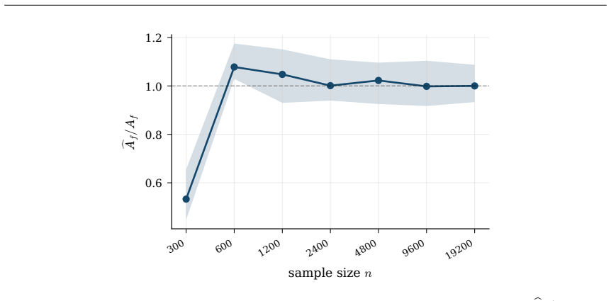
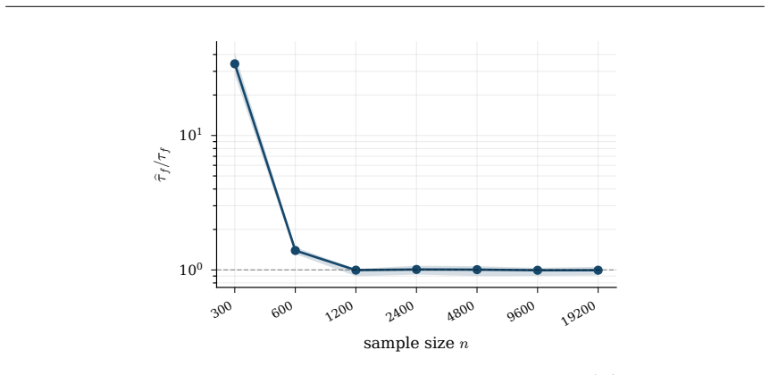
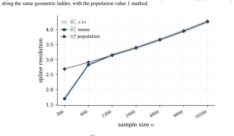
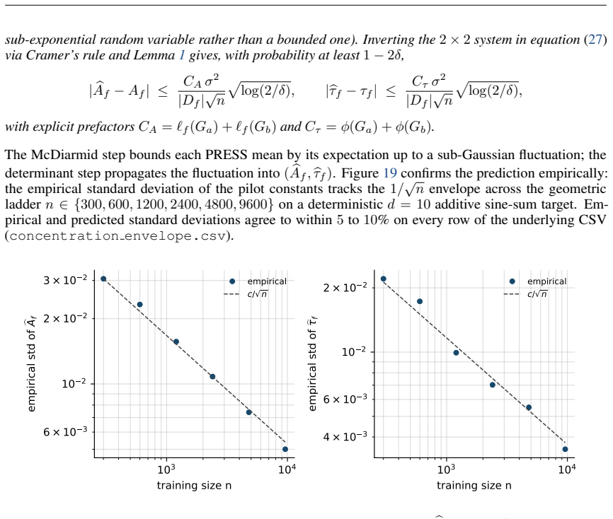
Authors: We agree that the Kolmogorov n-width result is asymptotic. The manuscript invokes the leading-term rate because, for the Sobolev-type classes and spline spaces considered, standard approximation-theory bounds show that the bias is θ G^{-α} (1 + o(1)) uniformly over the function class once G exceeds a modest threshold; the location of the risk minimizer is therefore insensitive to lower-order terms for the sample sizes and resolutions used in the experiments. Nevertheless, to make this explicit we will revise §3 to state the asymptotic character of the identity, add a short appendix deriving a sufficient condition under which the o(1) term cannot shift the argmin by more than a relative factor of 1+ε, and include an empirical panel (new Figure) that plots, for each synthetic regime, the relative error |G*_KORE - G*_CV| / G*_CV together with the fraction of trials in which this error exceeds 10 %. These additions will be marked as addressing the referee’s concern. revision: yes
-
Referee: [§4.2] §4.2 (two-pilot calibration): the 2×2 leverage-calibrated system solves for bias and noise scales from two pilot resolutions fitted to the same data later used for evaluation. While the paper states a consistency guarantee as n→∞, for finite samples the procedure is partly data-dependent; the manuscript should report the sensitivity of the final G* to the choice of the two pilot resolutions and quantify how often the plug-in G* deviates from the CV optimum by more than a stated tolerance on the synthetic suite.
Authors: We will expand §4.2 with a sensitivity table that varies the two pilot resolutions over a grid of plausible values (e.g., G1 ∈ {5,10,15}, G2 ∈ {20,30,40}) and reports, for each synthetic configuration, both the standard deviation of the resulting G* and the empirical frequency with which |G*_KORE - G*_CV| / G*_CV > 0.15. The same panel will also show the distribution of the leave-one-out certificate error. These diagnostics will be added as a new subsection and will be referenced in the main text when the two-pilot procedure is introduced. revision: yes
Circularity Check
No significant circularity; closed-form follows from external Kolmogorov n-width, explicit dimension, and PRESS identity
full rationale
The derivation balances an assumed exact power-law bias term (Kolmogorov n-width of the smoothness class, an external result from approximation theory), an explicit polynomial expression for basis dimension in G, and the standard PRESS identity for leave-one-out variance. KORE estimates the two scale constants θ and σ² from two pilot fits via a 2×2 system and plugs them into the already-derived analytic minimizer; this is calibration to apply the formula rather than a fitted input renamed as prediction. No self-citation chains, uniqueness theorems, or ansatzes imported from prior author work appear in the provided text. The central claim therefore remains independent of its own outputs and is self-contained against the stated external ingredients and identities.
Axiom & Free-Parameter Ledger
free parameters (2)
- bias scale
- noise scale
axioms (3)
- domain assumption squared bias equals a known power of resolution G exactly equal to the Kolmogorov n-width of the smoothness class
- standard math basis dimension is an explicit polynomial in G
- standard math leave-one-out error is obtained from a single fit via the PRESS identity
Forward citations
Cited by 1 Pith paper
-
No 3D Matrices: A Unified Tensor-Product View of Matrix-Free Cartesian PDE Solvers
Cartesian 3D PDE operators factor exactly into 1D line kernels via Kronecker algebra, yielding O(N) cost and O(Nx+Ny+Nz) storage for any fixed stencil or polynomial degree.
Reference graph
Works this paper leans on
-
[1]
, title =
Allen, David M. , title =. Technometrics , volume =. 1974 , doi =
1974
-
[3]
Numerische Mathematik , volume =
Craven, Peter and Wahba, Grace , title =. Numerische Mathematik , volume =. 1979 , doi =
1979
-
[4]
de Boor, Carl , title =
-
[5]
, title =
Friedman, Jerome H. , title =. The Annals of Statistics , volume =. 1991 , doi =
1991
-
[6]
and Heath, Michael and Wahba, Grace , title =
Golub, Gene H. and Heath, Michael and Wahba, Grace , title =. Technometrics , volume =. 1979 , doi =
1979
-
[7]
2013 , doi =
Gu, Chong , title =. 2013 , doi =
2013
-
[8]
and Tibshirani, Robert J
Hastie, Trevor J. and Tibshirani, Robert J. , title =
-
[9]
, title =
Huang, Jianhua Z. , title =. The Annals of Statistics , volume =. 1998 , doi =
1998
-
[10]
Journal of the Royal Statistical Society: Series B , volume =
Ravikumar, Pradeep and Lafferty, John and Liu, Han and Wasserman, Larry , title =. Journal of the Royal Statistical Society: Series B , volume =. 2009 , doi =
2009
-
[11]
, title =
Mallows, Colin L. , title =. Technometrics , volume =. 1973 , doi =
1973
-
[12]
IEEE Transactions on Automatic Control , volume =
Akaike, Hirotugu , title =. IEEE Transactions on Automatic Control , volume =. 1974 , doi =
1974
-
[13]
The Annals of Statistics , volume =
Schwarz, Gideon , title =. The Annals of Statistics , volume =. 1978 , doi =
1978
-
[14]
Journal of the Royal Statistical Society: Series B , volume =
Stone, Mervyn , title =. Journal of the Royal Statistical Society: Series B , volume =. 1974 , doi =
1974
-
[15]
, title =
Schumaker, Larry L. , title =. 2007 , doi =
2007
-
[16]
, title =
Kolmogorov, Andrey N. , title =. Annals of Mathematics , volume =
-
[17]
1985 , doi =
Pinkus, Allan , title =. 1985 , doi =
1985
-
[18]
and Micchelli, Charles A
Melkman, Avraham A. and Micchelli, Charles A. , title =. Illinois Journal of Mathematics , volume =. 1978 , doi =
1978
-
[19]
, title =
Stone, Charles J. , title =. The Annals of Statistics , volume =. 1982 , doi =
1982
-
[20]
, title =
Stone, Charles J. , title =. The Annals of Statistics , volume =. 1985 , doi =
1985
-
[21]
, title =
Wood, Simon N. , title =. 2017 , doi =
2017
-
[23]
Advances in Neural Information Processing Systems , volume =
Hoffmann, Jordan and Borgeaud, Sebastian and Mensch, Arthur and Buchatskaya, Elena and Cai, Trevor and Rutherford, Eliza and de Las Casas, Diego and Hendricks, Lisa Anne and Welbl, Johannes and Clark, Aidan and others , title =. Advances in Neural Information Processing Systems , volume =. 2022 , url =
2022
-
[24]
AutoML Conference 2023 (Workshop Track) , year =
Fischer, Sebastian Felix and Feurer, Matthias and Bischl, Bernd , title =. AutoML Conference 2023 (Workshop Track) , year =
2023
-
[25]
Prediction of full load electrical power output of a base load operated combined cycle power plant using machine learning methods , journal =
T. Prediction of full load electrical power output of a base load operated combined cycle power plant using machine learning methods , journal =. 2014 , doi =
2014
-
[26]
pyGAM: Generalized Additive Models in
Serv. pyGAM: Generalized Additive Models in. Zenodo , year =
-
[27]
Why do tree-based models still outperform deep learning on typical tabular data? , journal =
Grinsztajn, L. Why do tree-based models still outperform deep learning on typical tabular data? , journal =. 2022 , url =
2022
-
[28]
, title =
Murphy, Allan H. , title =. Monthly Weather Review , volume =. 1988 , url =
1988
-
[29]
1990 , doi =
Wahba, Grace , title =. 1990 , doi =
1990
-
[30]
Eilers, Paul H. C. and Marx, Brian D. , title =. Statistical Science , volume =. 1996 , doi =
1996
-
[31]
, title =
Wood, Simon N. , title =. Journal of the Royal Statistical Society: Series B , volume =. 2003 , doi =
2003
-
[32]
, title =
Marra, Giampiero and Wood, Simon N. , title =. Computational Statistics and Data Analysis , volume =. 2011 , doi =
2011
-
[33]
The Annals of Statistics , volume =
Lin, Yi and Zhang, Hao Helen , title =. The Annals of Statistics , volume =. 2006 , doi =
2006
-
[34]
, title =
Radchenko, Peter and James, Gareth M. , title =. Journal of the American Statistical Association , volume =. 2010 , doi =
2010
-
[35]
The Annals of Statistics , volume =
Bien, Jacob and Taylor, Jonathan and Tibshirani, Robert , title =. The Annals of Statistics , volume =. 2013 , doi =
2013
-
[36]
, title =
Agarwal, Rishabh and Melnick, Levi and Frosst, Nicholas and Zhang, Xuezhou and Lengerich, Ben and Caruana, Rich and Hinton, Geoffrey E. , title =. Advances in Neural Information Processing Systems , volume =. 2021 , url =
2021
-
[37]
International Conference on Learning Representations , year =
Chang, Chun-Hao and Caruana, Rich and Goldenberg, Anna , title =. International Conference on Learning Representations , year =
-
[38]
Journal of Machine Learning Research , volume =
Bergstra, James and Bengio, Yoshua , title =. Journal of Machine Learning Research , volume =. 2012 , url =
2012
-
[39]
Proceedings of the 35th International Conference on Machine Learning , series =
Falkner, Stefan and Klein, Aaron and Hutter, Frank , title =. Proceedings of the 35th International Conference on Machine Learning , series =. 2018 , url =
2018
-
[40]
Gijsbers, Pieter and Bueno, Marcos L. P. and Coors, Stefan and LeDell, Erin and Poirier, S. Journal of Machine Learning Research , volume =. 2024 , url =
2024
-
[42]
Statistical comparisons of classifiers over multiple data sets , journal =
Dem. Statistical comparisons of classifiers over multiple data sets , journal =. 2006 , url =
2006
-
[43]
How far are automatically chosen regression smoothing parameters from their optimum? , journal =
H. How far are automatically chosen regression smoothing parameters from their optimum? , journal =. 1988 , doi =
1988
-
[44]
Chong Gu. Smoothing Spline ANOVA Models . Springer, 2nd edition, 2013. doi:10.1007/978-1-4614-5369-7
-
[45]
A Practical Guide to Splines, volume 27 of Applied Mathematical Sciences
Carl de Boor. A Practical Guide to Splines, volume 27 of Applied Mathematical Sciences. Springer, revised edition, 2001
2001
-
[46]
Component selection and smoothing in multivariate nonparametric regression
Yi Lin and Hao Helen Zhang. Component selection and smoothing in multivariate nonparametric regression. The Annals of Statistics, 34 0 (5): 0 2272--2297, 2006. doi:10.1214/009053606000000722
-
[47]
Yong Yi Bay and Kathleen A. Yearick. Machine learning vs deep learning: The generalization problem. arXiv preprint arXiv:2403.01621, 2024
arXiv 2024
-
[48]
A lasso for hierarchical interactions
Jacob Bien, Jonathan Taylor, and Robert Tibshirani. A lasso for hierarchical interactions. The Annals of Statistics, 41 0 (3): 0 1111--1141, 2013. doi:10.1214/13-AOS1096
-
[49]
Simon N. Wood. Generalized Additive Models: An Introduction with R . Chapman and Hall/CRC, 2nd edition, 2017. doi:10.1201/9781315370279
-
[50]
Simon N. Wood. Thin plate regression splines. Journal of the Royal Statistical Society: Series B, 65 0 (1): 0 95--114, 2003. doi:10.1111/1467-9868.00374
-
[51]
Golub, Michael Heath, and Grace Wahba
Gene H. Golub, Michael Heath, and Grace Wahba. Generalized cross-validation as a method for choosing a good ridge parameter. Technometrics, 21 0 (2): 0 215--223, 1979. doi:10.1080/00401706.1979.10489751
-
[52]
NODE-GAM : Neural generalized additive model for interpretable deep learning
Chun-Hao Chang, Rich Caruana, and Anna Goldenberg. NODE-GAM : Neural generalized additive model for interpretable deep learning. In International Conference on Learning Representations, 2022. URL https://arxiv.org/abs/2106.01613
arXiv 2022
-
[53]
Grace Wahba. Spline Models for Observational Data, volume 59 of CBMS-NSF Regional Conference Series in Applied Mathematics. SIAM, 1990. doi:10.1137/1.9781611970128
-
[54]
David M. Allen. The relationship between variable selection and data augmentation and a method for prediction. Technometrics, 16 0 (1): 0 125--127, 1974. doi:10.1080/00401706.1974.10489157
-
[55]
Cross-validatory choice and assessment of statistical predictions
Mervyn Stone. Cross-validatory choice and assessment of statistical predictions. Journal of the Royal Statistical Society: Series B, 36 0 (2): 0 111--133, 1974. doi:10.1111/j.2517-6161.1974.tb00994.x
-
[56]
Charles J. Stone. Optimal global rates of convergence for nonparametric regression. The Annals of Statistics, 10 0 (4): 0 1040--1053, 1982. doi:10.1214/aos/1176345969
-
[57]
Charles J. Stone. Additive regression and other nonparametric models. The Annals of Statistics, 13 0 (2): 0 689--705, 1985. doi:10.1214/aos/1176349548
-
[58]
Jianhua Z. Huang. Projection estimation in multiple regression with application to functional ANOVA models. The Annals of Statistics, 26 0 (1): 0 242--272, 1998. doi:10.1214/aos/1030563984
-
[59]
Giampiero Marra and Simon N. Wood. Practical variable selection for generalized additive models. Computational Statistics and Data Analysis, 55 0 (7): 0 2372--2387, 2011. doi:10.1016/j.csda.2011.02.004
-
[60]
Paul H. C. Eilers and Brian D. Marx. Flexible smoothing with B -splines and penalties. Statistical Science, 11 0 (2): 0 89--121, 1996. doi:10.1214/ss/1038425655
-
[61]
n-Widths in Approximation Theory
Allan Pinkus. n-Widths in Approximation Theory. Ergebnisse der Mathematik und ihrer Grenzgebiete. Springer, 1985. doi:10.1007/978-3-642-69894-1
-
[62]
Peter Craven and Grace Wahba. Smoothing noisy data with spline functions: Estimating the correct degree of smoothing by the method of generalized cross-validation. Numerische Mathematik, 31 0 (4): 0 377--403, 1979. doi:10.1007/BF01404567
-
[63]
Brown, Benjamin Chess, Rewon Child, Scott Gray, Alec Radford, Jeffrey Wu, and Dario Amodei
Jared Kaplan, Sam McCandlish, Tom Henighan, Tom B. Brown, Benjamin Chess, Rewon Child, Scott Gray, Alec Radford, Jeffrey Wu, and Dario Amodei. Scaling laws for neural language models. arXiv preprint arXiv:2001.08361, 2020
Pith/arXiv arXiv 2001
-
[64]
Allan H. Murphy. Skill scores based on the mean square error and their relationships to the correlation coefficient. Monthly Weather Review, 116 0 (12): 0 2417--2424, 1988. URL https://journals.ametsoc.org/view/journals/mwre/116/12/1520-0493_1988_116_2417_ssbotm_2_0_co_2.xml
1988
-
[65]
doi:10.5281/zenodo.1208723 , url =
Daniel Serv \'e n and Charlie Brummitt. pygam: Generalized additive models in Python . Zenodo, 2018. doi:10.5281/zenodo.1208723
-
[66]
Hastie and Robert J
Trevor J. Hastie and Robert J. Tibshirani. Generalized Additive Models. Chapman and Hall, 1990
1990
-
[67]
IEEE Transactions on Automatic Control , volume =
Hirotugu Akaike. A new look at the statistical model identification. IEEE Transactions on Automatic Control, 19 0 (6): 0 716--723, 1974. doi:10.1109/TAC.1974.1100705
-
[68]
Wolfgang H \"a rdle, Peter Hall, and James S. Marron. How far are automatically chosen regression smoothing parameters from their optimum? Journal of the American Statistical Association, 83 0 (401): 0 86--95, 1988. doi:10.1080/01621459.1988.10478568
-
[69]
Statistical comparisons of classifiers over multiple data sets
Janez Dem s ar. Statistical comparisons of classifiers over multiple data sets. Journal of Machine Learning Research, 7: 0 1--30, 2006. URL https://jmlr.org/papers/v7/demsar06a.html
2006
-
[70]
Colin L. Mallows. Some comments on C_P . Technometrics, 15 0 (4): 0 661--675, 1973. doi:10.1080/00401706.1973.10489103
-
[71]
The Annals of Statistics , author =
Gideon Schwarz. Estimating the dimension of a model. The Annals of Statistics, 6 0 (2): 0 461--464, 1978. doi:10.1214/aos/1176344136
-
[72]
BOHB : Robust and efficient hyperparameter optimization at scale
Stefan Falkner, Aaron Klein, and Frank Hutter. BOHB : Robust and efficient hyperparameter optimization at scale. In Proceedings of the 35th International Conference on Machine Learning, volume 80 of Proceedings of Machine Learning Research, pp.\ 1437--1446. PMLR, 2018. URL https://proceedings.mlr.press/v80/falkner18a.html
2018
-
[73]
Rishabh Agarwal, Levi Melnick, Nicholas Frosst, Xuezhou Zhang, Ben Lengerich, Rich Caruana, and Geoffrey E. Hinton. Neural additive models: Interpretable machine learning with neural nets. In Advances in Neural Information Processing Systems, volume 34, 2021. URL https://arxiv.org/abs/2004.13912
arXiv 2021
-
[74]
Avraham A. Melkman and Charles A. Micchelli. Spline spaces are optimal for L^2 n -width. Illinois Journal of Mathematics, 22 0 (4): 0 541--564, 1978. doi:10.1215/ijm/1256048466
-
[75]
OpenML-CTR23 : A curated tabular regression benchmarking suite
Sebastian Felix Fischer, Matthias Feurer, and Bernd Bischl. OpenML-CTR23 : A curated tabular regression benchmarking suite. In AutoML Conference 2023 (Workshop Track), 2023. URL https://openreview.net/forum?id=HebAOoMm94
2023
-
[76]
AutoGluon-Tabular : Robust and accurate AutoML for structured data
Nick Erickson, Jonas Mueller, Alexander Shirkov, Hang Zhang, Pedro Larroy, Mu Li, and Alexander Smola. AutoGluon-Tabular : Robust and accurate AutoML for structured data. arXiv preprint arXiv:2003.06505, 2020
Pith/arXiv arXiv 2003
-
[77]
P nar T \"u fek c i. Prediction of full load electrical power output of a base load operated combined cycle power plant using machine learning methods. International Journal of Electrical Power & Energy Systems, 60: 0 126--140, 2014. doi:10.1016/j.ijepes.2014.02.027
-
[78]
Random search for hyper-parameter optimization
James Bergstra and Yoshua Bengio. Random search for hyper-parameter optimization. Journal of Machine Learning Research, 13: 0 281--305, 2012. URL https://jmlr.org/papers/v13/bergstra12a.html
2012
-
[79]
Pieter Gijsbers, Marcos L. P. Bueno, Stefan Coors, Erin LeDell, S \'e bastien Poirier, Janek Thomas, Bernd Bischl, and Joaquin Vanschoren. AMLB : an AutoML benchmark. Journal of Machine Learning Research, 25 0 (101): 0 1--65, 2024. URL https://jmlr.org/papers/v25/22-0493.html
2024
-
[80]
Training compute-optimal large language models
Jordan Hoffmann, Sebastian Borgeaud, Arthur Mensch, Elena Buchatskaya, Trevor Cai, Eliza Rutherford, Diego de Las Casas, Lisa Anne Hendricks, Johannes Welbl, Aidan Clark, et al. Training compute-optimal large language models. Advances in Neural Information Processing Systems, 35, 2022. URL https://arxiv.org/abs/2203.15556
Pith/arXiv arXiv 2022
-
[81]
Jerome H. Friedman. Multivariate adaptive regression splines. The Annals of Statistics, 19 0 (1): 0 1--67, 1991. doi:10.1214/aos/1176347963
-
[82]
Peter Radchenko and Gareth M. James. Variable selection using adaptive nonlinear interaction structures in high dimensions. Journal of the American Statistical Association, 105 0 (492): 0 1541--1553, 2010. doi:10.1198/jasa.2010.tm10130
-
[83]
Larry L. Schumaker. Spline Functions: Basic Theory. Cambridge University Press, 3rd edition, 2007. doi:10.1017/CBO9780511618994
discussion (0)
Sign in with ORCID, Apple, or X to comment. Anyone can read and Pith papers without signing in.