pith. sign in

arxiv: 2606.24937 · v1 · pith:JQPU726Qnew · submitted 2026-06-22 · 💻 cs.AI · cs.CL· cs.IR· cs.LG

The Hitchhiker's Guide to Agentic AI: From Foundations to Systems

Pith reviewed 2026-06-26 08:08 UTC · model grok-4.3

classification 💻 cs.AI cs.CLcs.IRcs.LG
keywords agentic AILLM foundationsRLHFRAGmulti-agent systemsAI deploymentreasoning models
0
0 comments X

The pith

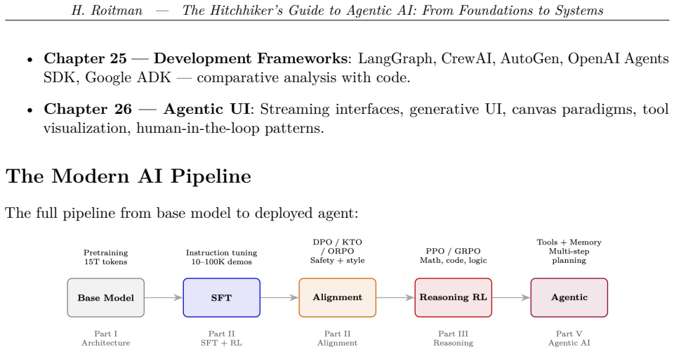
Effective agentic AI systems require understanding every layer of the development pipeline from model foundations to multi-agent coordination.

A machine-rendered reading of the paper's core claim, the machinery that carries it, and where it could break.

This guide to agentic AI argues that successful autonomous systems emerge only when developers master the complete stack rather than specializing in isolated components. It details the LLM substrate including transformers and optimization techniques, then moves to alignment methods like RLHF and reasoning enhancements, before covering agent-specific elements such as RAG, memory systems, harness design, and inter-agent protocols. A reader would care because fragmented approaches often result in brittle or inefficient agents, while an integrated view supports scalable production deployments. The work pairs theoretical explanations with implementation details to bridge research and practice.

Core claim

The central claim is that building great agentic systems requires understanding every layer of the pipeline, not just one. The book treats the LLM substrate, alignment and reasoning layers, agentic training and retrieval methods, memory and harness design, inter-agent communication protocols, and production frameworks as interdependent components that must be addressed together for effective autonomous AI.

What carries the argument

The full pipeline architecture spanning LLM foundations, alignment techniques, agent design patterns, and A2A coordination protocols.

If this is right

  • Agentic training using trajectory-based RL becomes necessary alongside standard fine-tuning for advanced capabilities.
  • Retrieval-augmented generation must be extended to Agentic RAG to handle dynamic agent needs.
  • Multi-agent architectures benefit from standardized protocols like MCP and A2A for reliable coordination.
  • Evaluation methodologies need to assess full agent trajectories and interactions rather than isolated outputs.
  • Production deployment requires attention to context management and UI design integrated with the core model.

Where Pith is reading between the lines

These are editorial extensions of the paper, not claims the author makes directly.

  • Developers might benefit from modular training programs that cover the stack sequentially rather than in silos.
  • This synthesis could accelerate the shift from single-model applications to orchestrated agent teams in industry.
  • Future work might test whether omitting any single layer leads to measurable drops in agent reliability.
  • The guide's structure implies that rapid field changes will require ongoing updates to maintain relevance.

Load-bearing premise

A single comprehensive synthesis of techniques from disparate AI subfields can be created and remain useful despite their fast pace of change.

What would settle it

A controlled comparison where teams build agents using only partial pipeline knowledge versus the full integrated guide, measuring differences in task success rates and robustness.

Figures

Figures reproduced from arXiv: 2606.24937 by Haggai Roitman.

Figure 1
Figure 1. Figure 1: The modern LLM development pipeline: from pre-trained base model through alignment and reasoning to autonomous agentic capability. Each stage maps to a part of this guide. 33 [PITH_FULL_IMAGE:figures/full_fig_p033_1.png] view at source ↗
Figure 1.1
Figure 1.1. Figure 1.1: The LLM pipeline: text is tokenized into subword units, converted to integer IDs, embedded as dense vectors, processed through transformer layers, projected to vocabulary logits, and decoded back to text. The dashed loop shows autoregressive generation—each output token is appended to the input for the next forward pass. The Four Key Stages 1. Tokenization: Raw text is split into subword pieces (not char… view at source ↗
Figure 1.2
Figure 1.2. Figure 1.2: BPE tokenization example: starting from characters, the algorithm iteratively merges the most frequent adjacent pairs until the word becomes a single token or the vocabulary budget is exhausted. 36 [PITH_FULL_IMAGE:figures/full_fig_p036_1_2.png] view at source ↗
Figure 1.3
Figure 1.3. Figure 1.3: Decoder-only Transformer block (GPT-style, Pre-Norm variant). Each sub-layer (attention, FFN) is preceded by LayerNorm and followed by a residual addition: x + SubLayer(LN(x)). This Pre-Norm ordering (used by Llama, GPT-3, Mistral) stabilizes training without warmup, unlike the original Post-Norm (which applies LayerNorm after the addition). L identical blocks are stacked, followed by a final LayerNorm a… view at source ↗
Figure 1.4
Figure 1.4. Figure 1.4: The original Transformer architecture (Vaswani et al., 2017). The encoder (left) processes the full input with bidirectional self-attention. The decoder (right) generates tokens autoregressively using masked self-attention and cross-attention to encoder representations. Dashed boxes indicate the repeated layer block (×N); gray lines show residual connections bypassing each sub-layer. Note: the original w… view at source ↗
Figure 1.5
Figure 1.5. Figure 1.5: Embedding space visualization (2D projection): semantically similar words cluster together. The embedding table learns these positions during pretraining, capturing meaning purely from co-occurrence patterns in text. Why Embeddings Work The embedding table is learned end-to-end with the rest of the model. Because the model is trained to predict the next token, it must learn representations where tokens t… view at source ↗
Figure 1.6
Figure 1.6. Figure 1.6: Isotropy vs. anisotropy in embedding spaces. Left: isotropic embeddings spread uniformly, making cosine similarity a reliable measure of semantic relatedness. Right: anisotropic embeddings (as found in BERT) cluster in a narrow cone, causing all pairs to have high cosine similarity regardless of semantic content. Whitening transforms the space to restore isotropy. Whitening in Practice • What it does: Ro… view at source ↗
Figure 1.7
Figure 1.7. Figure 1.7: The same transformer backbone supports different tasks by swapping the prediction head. All three heads used in this paper share identical architecture below the final projection layer. P(xt+1|x≤t) = softmax(Whead · ht + b) (1.7) where Whead ∈ R |V|×d (often tied with the embedding matrix: Whead = ET ). LM Head Properties • Training objective: Causal language modeling (predict next token for every positi… view at source ↗
Figure 1.8
Figure 1.8. Figure 1.8: Gradient descent: starting from a random initialization θ0, each step moves the parameters in the direction that reduces the loss, with step size controlled by the learning rate η. The process converges toward a (local) minimum. Why Full Gradient Descent is Impractical. Computing the exact gradient requires evaluating the loss over the entire training dataset (trillions of tokens for LLMs). This is compu… view at source ↗
Figure 1.9
Figure 1.9. Figure 1.9: Common learning rate schedules. All include a linear warmup phase. WSD (Warmup-Stable￾Decay) is the emerging standard for pretraining. (a) Constant. Simplest schedule. Good for short fine-tuning runs where you want to avoid over-decaying the LR. Risk: no annealing means the model may not converge to the sharpest minimum. 61 [PITH_FULL_IMAGE:figures/full_fig_p061_1_9.png] view at source ↗
Figure 1.10
Figure 1.10. Figure 1.10: LoRA decomposes the weight update ∆W into two small matrices B × A. The original weight W remains frozen; only B and A receive gradients. At inference, the product BA can be merged into W with zero overhead. Why the α/r Scaling Matters Without scaling, doubling the rank r would roughly double the magnitude of ∆W = BA (more columns in B contribute to the sum). This means changing rank would also change h… view at source ↗
Figure 1.11
Figure 1.11. Figure 1.11: MoE layer with 8 experts and Top-2 routing. Only the two highest-gated experts are computed per token; the rest are skipped entirely. 1.10.2 Load Balancing The Load Balancing Problem Without constraints, the router may send most tokens to the same 1–2 experts (“expert collapse”). This wastes capacity and creates compute imbalance across GPUs (each expert typically lives on a different GPU). Solution: Ad… view at source ↗
Figure 1.12
Figure 1.12. Figure 1.12: Beam search with B = 2. At each step, only the 2 highest-scoring partial sequences survive (blue). Lower-scoring alternatives are pruned (gray). 1.12.3 Diverse Beam Search Standard beam search produces near-duplicate beams. Diverse beam search [112] partitions beams into G groups and adds a dissimilarity penalty between groups: scoreg(yt) = log P(yt |y<t) − λ X g ′<g ∆(yt , Yg ′) where ∆ measures overla… view at source ↗
Figure 1.13
Figure 1.13. Figure 1.13: Top-p (nucleus) sampling: tokens are sorted by probability and included until cumulative mass reaches p = 0.9. The nucleus (dark blue) adapts its size to the distribution shape — here 5 tokens suffice. Top-kk vs. Top-pp Consider predicting the next word: • After “2 + 2 =”: distribution is peaked — top-1 token (“4”) has 99% mass. Top-k=50 wastefully considers 49 wrong answers. Top-p=0.9 correctly picks j… view at source ↗
Figure 1.14
Figure 1.14. Figure 1.14: Safety is applied at every stage: data filtering in pretraining, refusal examples in SFT, safety￾specific reward models in RLHF, and iterative red-teaming. 1.17.3 Key Safety Mechanisms Safety Techniques • Data filtering: Remove toxic, biased, and PII-containing text from pretraining corpora • Safety SFT: Train on examples of appropriate refusals (“I can’t help with that because. . . ”) • Constitutional … view at source ↗
Figure 2.1
Figure 2.1. Figure 2.1: Left: Internal structure of a single Streaming Multiprocessor (SM) on A100 — 64 FP32 CUDA cores, 4 Tensor Cores, 4 warp schedulers, 256 KB register file, and 192 KB shared memory/L1 cache. Right: The full A100 chip contains 108 SMs with shared 40 MB L2 cache and 80 GB HBM2e. Bandwidth annotations (left margin) show the dramatic drop from registers to HBM. 106 [PITH_FULL_IMAGE:figures/full_fig_p106_2_1.png] view at source ↗
Figure 2.2
Figure 2.2. Figure 2.2: Roofline model for A100 BF16. Attention is deep in the memory-bound regime; large GEMMs (FFN layers) are compute-bound. • Read S for softmax: n 2 × 2 = 33.5 MB • Write softmax output P: n 2 × 2 = 33.5 MB • Read P and V for final matmul: n 2 × 2 + n × d × 2 = 34.5 MB • Write output O: n × d × 2 = 1 MB Total memory: ≈ 138 MB (dominated by 4 passes over the n 2 attention matrix). Arithmetic intensity: I = 8… view at source ↗
Figure 2.3
Figure 2.3. Figure 2.3: Two-node 8-GPU topology. Intra-node: NVLink 4 via NVSwitch (900 GB/s total). Inter-node: InfiniBand NDR 400Gb/s via top-of-rack switch. Each node has 8 IB NICs (one per GPU) for rail-optimized AllReduce. Choosing Parallelism Based on Bandwidth • Tensor Parallelism (TP): Requires all-reduce every layer – use only within a node over NVLink. TP=8 is standard for H100 DGX nodes. • Pipeline Parallelism (PP): … view at source ↗
Figure 2.4
Figure 2.4. Figure 2.4: vLLM architecture: Requests flow top-down. The Scheduler manages admission and preemption, the Block Manager handles virtual-to-physical KV cache mapping (like OS page tables), and the Model Executor runs batched inference reading from the pre-allocated block pool in GPU HBM. • Block Manager: Implements the virtual memory abstraction for KV caches. Maps logical blocks (per-sequence) to physical blocks (i… view at source ↗
Figure 3.1
Figure 3.1. Figure 3.1: Reinforcement Learning overview: an agent interacts with an environment, receiving rewards as feedback and updating its policy through trial and error. Unlike supervised learning which learns from labeled pairs, RL learns what to do by maximizing reward through experience. 3.1 The Markov Decision Process (MDP) An MDP is a 5-tuple (S, A, P, R, γ): • S: State space — all possible configurations of the envi… view at source ↗
Figure 3.2
Figure 3.2. Figure 3.2: GAE data flow: each TD residual δ V t+l is weighted by (γλ) l before summation. Higher λ includes more future residuals (lower bias, higher variance). What λ Controls — Bias-Variance Tradeoff • λ = 0: Aˆ t = δt = rt + γV (st+1) − V (st). Trust value function completely. Low variance, but biased if V is inaccurate. • λ = 1: Aˆ t = P l γ l rt+l − V (st). Full Monte Carlo return minus baseline. Unbiased but… view at source ↗
Figure 3.3
Figure 3.3. Figure 3.3: Bias vs. Variance in GAE: λ controls the trade-off. Small λ (left) yields high bias / low variance via bootstrapping; large λ (right) yields low bias / high variance using full Monte Carlo returns. The optimal choice (λ ∈ [0.9, 0.95]) balances stable training with accurate long-horizon credit assignment. The hyperparameter λ serves as a slide-rule between two fundamental estimation paradigms. High Bias /… view at source ↗
Figure 5.1
Figure 5.1. Figure 5.1: PPO end-to-end: from prompt batch through generation, reward scoring, KL computation, advantage estimation, to clipped policy update. The feedback loop shows the updated policy being used for the next generation step. Core Architecture: Two Networks 1. The Policy Network (πθ): The active, live network parameterized by weights θ. Continu￾ously updated via backpropagation during optimization. 2. The Old Po… view at source ↗
Figure 7.1
Figure 7.1. Figure 7.1: GRPO in action: G=5 responses are sampled for a single math prompt. Three are correct (r=1), two are wrong (r=0). The group mean µG=0.6 acts as the baseline; correct responses receive positive advantage (reinforced), wrong ones receive negative advantage (suppressed). 7.3 TRL Implementation The following shows a minimal working example using HuggingFace TRL. from trl import GRPOConfig , GRPOTrainer from … view at source ↗
Figure 8.1
Figure 8.1. Figure 8.1: Approximate quality vs. compute frontier. Methods above the SFT ceiling line improve beyond what supervised fine-tuning alone achieves. Position is illustrative and model-dependent. Decision Tree: Which Method to Use? 1. Do you have verifiable rewards? (math/code) → GRPO 2. Do you need max quality on complex tasks? → PPO 3. Do you have paired preferences? → DPO (or IPO if noisy) 4. Only unpaired binary f… view at source ↗
Figure 11.1
Figure 11.1. Figure 11.1: 70B PPO memory budget: the four models required for RLHF and their memory footprints. Total: 1470–1560GB. Minimum 19–20 A100-80GB (naive). With ZeRO-3: fits in 8 nodes. Memory Budget Reality Check – 70B BF16 Policy weights (BF16) 140 GB FP32 master weights 280 GB Adam optimizer (m + v, FP32) 560 GB Gradients (BF16) 140 GB Reference model 140 GB (or 70 GB in INT8) Reward model 140 GB (or 70 GB in INT8) A… view at source ↗
Figure 11.2
Figure 11.2. Figure 11.2: Overview of the four parallelism strategies. Production systems typically combine 2–3 of these simultaneously. 11.2.1 Data Parallelism (DP) and Distributed Data Parallelism (DDP) Data Parallelism is the simplest and most common form of distributed training [205]. Each GPU holds a complete copy of the model, processes a different mini-batch, and synchronizes gradients. Vanilla DP (PyTorch DataParallel). … view at source ↗
Figure 11.3
Figure 11.3. Figure 11.3: DDP: each GPU holds a full model replica and processes a different batch. Gradients are averaged via ring AllReduce, overlapped with backward computation. Key properties of DDP: • Memory: Each GPU stores full model + optimizer + gradients. For 70B BF16: ∼560 GB/GPU— impossible without memory optimizations. • Communication: One AllReduce of gradient tensor per step. Size = model parameters × 2 bytes (BF1… view at source ↗
Figure 11.4
Figure 11.4. Figure 11.4: Column-parallel linear layer (TP=2). The weight is split column-wise; each GPU computes XWi independently. The MLP pairs this with a row-parallel layer to avoid redundant AllReduce. 201 [PITH_FULL_IMAGE:figures/full_fig_p201_11_4.png] view at source ↗
Figure 11.5
Figure 11.5. Figure 11.5: Tensor Parallel communication pattern in one Transformer block. Two AllReduce operations (marked in red) are required per layer—one after attention, one after MLP. Why TP is Restricted to Intra-Node Each transformer layer requires 2 AllReduce operations (marked as f and g above). For a 70B model with 80 layers, that’s 160 AllReduce operations per forward pass (320 including backward). At NVLink speeds (… view at source ↗
Figure 11.6
Figure 11.6. Figure 11.6: Sequence Parallelism reduces activation memory for LayerNorm/Dropout by splitting along the sequence dimension. Communication (AllGather/ReduceScatter) replaces the AllReduce used in standard TP—same total bytes transferred, but memory is saved. SP Communication is “Free” Standard TP uses AllReduce after each sub-layer, which is equivalent to ReduceScatter + AllGather. SP simply reorders these primitive… view at source ↗
Figure 11.7
Figure 11.7. Figure 11.7: Pipeline bubble comparison. Left: naive pipeline with one micro-batch has 75% idle time. Right: GPipe with M = 4 micro-batches reduces bubbles significantly. With M ≫ P, bubble fraction approaches zero. Bubble Fraction Formula. For P pipeline stages and M micro-batches per step: Bubble fraction = P − 1 P + M − 1 ≈ P − 1 M (when M ≫ P) (11.3) To keep bubble overhead <10%, you need M ≥ 10 · (P − 1). For P… view at source ↗
Figure 11.8
Figure 11.8. Figure 11.8: FSDP shards all model state across GPUs. Each GPU owns 1/N of parameters, optimizer states, and gradients. Full parameters are reconstructed on-demand via AllGather before each layer’s computation. FSDP execution flow per layer: 1. Forward: AllGather parameters → compute → discard non-owned shards. 2. Backward: AllGather parameters (again) → compute gradients → ReduceScatter gradients (each GPU gets its… view at source ↗
Figure 11.9
Figure 11.9. Figure 11.9: 3D parallelism layout for 16 GPUs: TP=4 (within each box, using NVLink), PP=2 (orange arrows, stages), DP=2 (red arrows, gradient sync). Each dimension exploits a different level of the communi￾cation hierarchy. Decision flowchart: 1. Does the model fit on 1 GPU? → Use DDP. 2. Does it fit on 1 node with FSDP? → Use FSDP (ZeRO-3). 3. Does it fit on 1 node with TP+FSDP? → Use TP (intra-node) + FSDP (inter… view at source ↗
Figure 11.10
Figure 11.10. Figure 11.10: Decoupled RLHF architecture. Each cluster optimized for its workload. Scored rollouts accumulate in the experience buffer before being consumed by training. • Generation cluster is stateless → trivial fault tolerance • Can overlap gen(step N + 1) with training(step N) → 30–40% speedup • Different quantization: INT8 for generation (bandwidth), BF16 for training (precision) 11.5 Weight Synchronization St… view at source ↗
Figure 11.11
Figure 11.11. Figure 11.11: Without overlap (monolithic). With decoupled: gen overlaps with training, effective 1.4× speedup. Phase Time (70B) Bound By Optimization Generation (128×512 tok) 30–45s Memory bandwidth vLLM, spec decoding, INT8 Reward scoring 5–8s Compute (batch for￾ward) INT8 RM, batch=128 Reference log-probs 4–6s Compute (batch for￾ward) INT8 ref, or LoRA (free) PPO update (4 epochs) 8–12s Compute (backprop) FSDP, F… view at source ↗
Figure 12.1
Figure 12.1. Figure 12.1: From Chatbots to Autonomous Agents: Traditional LLM chatbots operate in a single-step conversational loop with immediate human feedback. Autonomous agents plan across multiple tool interactions, receive feedback from real-world execution environments, and optimize for sparse terminal rewards (task success/failure). The key differences that demand new RL approaches: • Multi-step reasoning: Agents must pl… view at source ↗
Figure 12.2
Figure 12.2. Figure 12.2: Productivity co-pilot architecture: the LLM agent (with RL policy πθ) receives user intents and interacts with multiple application APIs. A reward signal based on task success, user feedback, and efficiency metrics drives policy improvement. 12.6.2 Formal MDP Definition for a Productivity Co-pilot The productivity co-pilot environment is formalized as a Partially Observable Markov Decision Process (POMD… view at source ↗
Figure 13.1
Figure 13.1. Figure 13.1: Schematic test-time compute scaling curves. Performance improves log-linearly with inference tokens across model sizes, and smaller models with more compute can approach larger models with less compute. The practical implication is profound: reasoning models trade training compute for inference compute. Rather than always deploying the largest possible model, one can deploy a smaller, reasoning-capable … view at source ↗
Figure 13.2
Figure 13.2. Figure 13.2: Spectrum of test-time scaling methods. Each method trades additional inference compute for improved reasoning accuracy. Methods build on each other conceptually: CoT introduces explicit reasoning, Self-Consistency adds sampling, ToT adds structured search, GoT adds merging operations, and MCTS adds learned value guidance. 13.2.1 Chain-of-Thought (CoT) Chain-of-Thought prompting [122] is the foundation o… view at source ↗
Figure 13.3
Figure 13.3. Figure 13.3: Tree-of-Thoughts on the “Game of 24” task: use operations on 4, 9, 10, 13 to make 24. At each level, the model generates b = 3 candidate thoughts, evaluates each (sure/maybe/impossible), prunes unpromising branches, and expands the most promising ones. The green path leads to a solution; red paths are pruned early. 5. Repeat until a solution is found or depth limit reached DFS (Depth-First Search): 1. G… view at source ↗
Figure 13.4
Figure 13.4. Figure 13.4: Comparison of CoT (linear chain), ToT (tree — branches but no merging), and GoT (DAG — branches can merge). For a sorting task, GoT can split the array into sub-problems, solve them independently (parallel), then merge the results — impossible in a pure tree structure. This enables divide-and-conquer reasoning. Graph Operations (formal). Let V = {v1, . . . , vn} be thought vertices and E ⊆ V ×V be direc… view at source ↗
Figure 13.5
Figure 13.5. Figure 13.5: Four phases of MCTS for reasoning: (1) Selection: traverse tree using UCB to find a promising leaf; (2) Expansion: generate new reasoning steps from the leaf; (3) Simulation: complete the reasoning to a terminal state and evaluate; (4) Backpropagation: update value estimates along the path. • Generate 3 candidate first steps: 1. “Assume for contradiction that √ 2 = p/q in lowest terms.” (P = 0.7) 2. “Co… view at source ↗
Figure 15.1
Figure 15.1. Figure 15.1: The Agentic AI architecture stack. The Agent Core executes a perceive–reason–act loop, coordinated by the Harness & Orchestration layer which manages context, state, guardrails, and observ￾ability. The agent interacts downward with External Systems—RAG for knowledge retrieval, Memory for persistence, Tools via MCP, and other Agents via A2A—all grounded in an Environment. The User provides goals, feedbac… view at source ↗
Figure 16.1
Figure 16.1. Figure 16.1: End-to-end RAG architecture. The offline pipeline (blue) indexes documents once; the online pipeline (green/orange) serves each query at inference time. 16.2.2 Indexing Pipeline Document Loading. Documents arrive in heterogeneous formats (PDF, HTML, Markdown, DOCX, code). Loaders extract clean text and preserve metadata (source URL, page number, section title, timestamp) that will be stored alongside em… view at source ↗
Figure 16.2
Figure 16.2. Figure 16.2: Agentic RAG control flow. The agent iteratively plans, retrieves, evaluates sufficiency, and self-checks grounding before returning an answer. 16.7.3 Multi-Source Routing An agentic RAG system can route sub-queries to specialized knowledge sources. The core insight is that different question types demand different retrieval backends—no single index excels at everything. Why Route? Consider a financial a… view at source ↗
Figure 17.1
Figure 17.1. Figure 17.1: Four-way taxonomy of agentic memory systems, mirroring cognitive science distinctions. Each memory type has distinct access patterns, update frequencies, and retrieval mechanisms. 17.2 Taxonomy of Memory Types 17.2.1 Working Memory (Short-Term) Working memory is the agent’s active workspace: the information currently being manipulated. In LLM agents it corresponds to: • Scratchpads. Intermediate reasoni… view at source ↗
Figure 18.1
Figure 18.1. Figure 18.1: High-level architecture of an agent harness. The LLM handles only reasoning; all execution, memory, routing, and observability are managed by the harness. 18.2 Context Window Management The context window is the agent’s working memory. Every token in the window costs money and latency; every token not in the window is invisible to the model. Managing this finite resource is one of the most consequential… view at source ↗
Figure 18.2
Figure 18.2. Figure 18.2: Three sliding-window strategies. Red = pinned, gray = dropped, blue = retained verbatim, yellow = summarized, green = new message. where the root model partitions the context C into chunks {Ci}, formulates sub-queries {qi}, spawns recursive calls to process each chunk, and then synthesizes the results into a final answer. No single call ever sees the full context—the model manages what to examine at eac… view at source ↗
Figure 18.3
Figure 18.3. Figure 18.3: Recursive Language Model (RLM). The root model partitions the context into chunks, spawns sub-LLM calls at depth 1, which may recurse further (depth 2). Results flow back up (dashed green arrows) and are aggregated into a final answer. No single call processes the full context. 18.2.6 Token Counting and Budget Monitoring Pre-Flight Token Check Before every LLM call, the harness must: 1. Count tokens in … view at source ↗
Figure 18.4
Figure 18.4. Figure 18.4: MCP architecture. The harness acts as an MCP client, routing tool calls to specialized MCP servers over standardized transports. 18.5 Orchestration Patterns Orchestration defines how the agent decides what to do next. Different patterns suit different task structures. 18.5.1 ReAct Loop (Reason + Act) The ReAct pattern [127] interleaves reasoning (“Thought”) with action (“Act”) and observation (“Observe”… view at source ↗
Figure 18.5
Figure 18.5. Figure 18.5: ReAct loop: the agent alternates between reasoning and acting until a termination condition is met. Implementation Details. • The “Thought” step is typically a scratchpad—a chain-of-thought reasoning trace [122] that is not shown to the user. 353 [PITH_FULL_IMAGE:figures/full_fig_p353_18_5.png] view at source ↗
Figure 18.6
Figure 18.6. Figure 18.6: Supervisor pattern: one orchestrator routes to specialist agents. Peer-to-Peer. Agents communicate directly without a central coordinator. Each agent can invoke any other agent as a tool. Flexible but harder to debug and prone to circular dependencies. Hierarchical (Tree of Agents). A tree structure where high-level agents delegate to mid-level agents, which delegate to leaf agents. Enables recursive ta… view at source ↗
Figure 18.7
Figure 18.7. Figure 18.7: Example workflow graph for a human-in-the-loop agent. States and conditional transitions are explicit, making the control flow auditable. 18.6.1 Conversation State The message history is the primary state artifact. Each message has: • Role: system, user, assistant, tool. • Content: Text, tool call, or tool result. • Metadata: Timestamp, token count, importance score, compression status. 18.6.2 Task Stat… view at source ↗
Figure 19.1
Figure 19.1. Figure 19.1: Prompt chaining with quality gates. Each step is a separate LLM call. Gates can be LLM-based or programmatic. When to use: Tasks that are naturally sequential—content generation, data transformation, multi-stage analysis. Key advantage: Each step can use a different prompt, model, or temperature. Intermediate results are inspectable and debuggable. 369 [PITH_FULL_IMAGE:figures/full_fig_p369_19_1.png] view at source ↗
Figure 19.2
Figure 19.2. Figure 19.2: Routing pattern: input is classified once, then handled by a specialist. When to use: Distinct task types with different optimal prompts, tools, or models. Customer support triage, multi-modal input handling. 19.1.3 Parallelization Multiple LLM calls run concurrently, with a programmatic layer combining their outputs. Two sub-patterns emerge: • Sectioning (fan-out): Partition the input into disjoint chu… view at source ↗
Figure 19.3
Figure 19.3. Figure 19.3: Orchestrator-workers: the LLM decides how to decompose the task and synthesizes worker results [PITH_FULL_IMAGE:figures/full_fig_p371_19_3.png] view at source ↗
Figure 19.4
Figure 19.4. Figure 19.4: Evaluator-optimizer: iterative refinement without training. 19.2 Autonomous Agent Patterns These patterns give the LLM control over the execution flow itself. 19.2.1 ReAct (Reason + Act) The foundational agent pattern [127]. The LLM alternates between thinking (internal reasoning), acting (tool calls), and observing (processing results) in a loop until it produces a final answer. ReAct Implementation Es… view at source ↗
Figure 20.1
Figure 20.1. Figure 20.1: OpenEnv architecture with an LLM agent. The agent reasons via a harness loop, which calls the typed EnvClient. The client communicates over WebSocket to an HTTPEnvServer running inside a Docker container. An RL trainer (dashed) optionally wraps the loop to collect rollouts and reward signals for policy optimization. 20.4.1 Standardized Agent–Environment Interface OpenEnv defines a typed interface for ag… view at source ↗
Figure 20.2
Figure 20.2. Figure 20.2: Four agent–environment interface patterns. (a) Text-based is the most common for LLMs. (b) Structured JSON enables precise parsing. (c) Multimodal combines screenshots with accessibility trees for GUI tasks. (d) Streaming supports real-time interaction without discrete turn boundaries. Text-Based Observation/Action. The agent receives a string observation and produces a string action. The environment pa… view at source ↗
Figure 21.1
Figure 21.1. Figure 21.1: How MCP works: a single user request flows through the Host, LLM, and MCP Server. The LLM decides which tool to call (step 3); the Host routes the call to the appropriate server via JSON-RPC (step 4); the result flows back through the LLM for natural-language formatting (steps 5–7). The user never sees the protocol machinery. 21.2 Architecture Overview MCP follows a client-server architecture with three… view at source ↗
Figure 21.2
Figure 21.2. Figure 21.2: illustrates the full MCP stack, from the user interface down to external services [PITH_FULL_IMAGE:figures/full_fig_p395_21_2.png] view at source ↗
Figure 23.1
Figure 23.1. Figure 23.1: Combined A2A + MCP architecture. The orchestrator delegates to specialist agents via A2A; each agent accesses its tools via MCP servers. • A2A for delegation: When an agent needs capabilities it doesn’t have, it delegates to another agent via A2A task messages. Each agent is a self-contained service with its own Agent Card. • MCP for tool access: Each agent connects to its tools through MCP servers. Thi… view at source ↗
Figure 24.1
Figure 24.1. Figure 24.1: Centralized (Supervisor) architecture. The manager delegates tasks to specialized workers and aggregates their outputs. All communication flows through the central hub. The manager’s responsibilities include: • Task routing: deciding which worker is best suited for each sub-task • Context management: providing each worker with the relevant subset of global context • Result aggregation: synthesizing work… view at source ↗
Figure 24.2
Figure 24.2. Figure 24.2: Decentralized (peer-to-peer) architecture. Agents communicate directly; coordination emerges from local interactions. • Negotiation: agents bid for tasks or resources • Stigmergy: agents modify shared state that others observe (see Section 24.3.6) • Gossip protocols: agents propagate information through the network • Local consensus: small groups of agents reach agreement without global coordination Dec… view at source ↗
Figure 24.3
Figure 24.3. Figure 24.3: Hierarchical architecture. A top-level orchestrator delegates to domain sub-managers, who delegate to specialized workers. Dashed arrow shows an escalation path. The enterprise analogy is apt: a CEO (top orchestrator) sets strategy; VPs (sub-managers) translate strategy into domain plans; individual contributors (workers) execute. The hierarchy enables scale while preserving accountability. 24.2.4 Swarm… view at source ↗
Figure 25.1
Figure 25.1. Figure 25.1: illustrates the five major phases [PITH_FULL_IMAGE:figures/full_fig_p460_25_1.png] view at source ↗
Figure 25.2
Figure 25.2. Figure 25.2: LangGraph execution graph for the research agent. Conditional edges implement the tool-use loop and error handling. 25.3.2 AutoGen (Microsoft) AutoGen [338], developed by Microsoft Research, takes a fundamentally different approach: it models agents as conversable entities that communicate through structured message passing. Rather than a single agent loop, AutoGen enables multi-agent conversations wher… view at source ↗
Figure 25.3
Figure 25.3. Figure 25.3: Modular agent architecture. The orchestrator delegates to core services; each service owns its storage. Dashed lines show optional cross-service communication. 25.4.2 Key Open-Source Building Blocks Prompt Management. • Promptflow1 (Microsoft): Visual prompt engineering and evaluation • Guidance2 (Microsoft): Constrained generation with interleaved code and prompts 1 https://github.com/microsoft/promptf… view at source ↗
Figure 25.4
Figure 25.4. Figure 25.4: Agent testing pyramid. Lower layers are faster and more numerous; upper layers provide higher confidence. 25.5.1 Unit Testing Individual Tools Each tool should be tested in isolation with a comprehensive suite covering happy paths, error cases, and edge cases: import pytest from unittest . mock import patch , MagicMock from myagent . tools import search_web , read_document class TestSearchWebTool : def … view at source ↗
Figure 25.5
Figure 25.5. Figure 25.5: Queue-based async agent deployment. Workers pull tasks from a queue and persist state independently. from celery import Celery from myagent import ResearchAgent import redis import time app = Celery (" agent_tasks ", broker =" redis :// localhost :6379/0 ") state_store = redis . Redis ( host =" localhost ", port =6379 , db =1) @app . task ( bind = True , max_retries =3 , default_retry_delay =60) def run… view at source ↗
read the original abstract

The Hitchhiker's Guide to Agentic AI is a comprehensive practitioner's reference for building autonomous AI systems. The book covers the full stack from first principles to production deployment, organized around a central thesis: building great agentic systems requires understanding every layer of the pipeline, not just one. The book opens with the LLM substrate -- transformer architecture, GPU systems, training and fine-tuning (SFT,LoRA, MoE), model compression, and inference optimization -- treated as essential foundations rather than the primary focus. It then develops the alignment and reasoning layer: reinforcement learning from human feedback (RLHF), PPO, DPO and its variants, GRPO, reward modeling, and RL for large reasoning models including chain-of-thought and test-time scaling. The second half is devoted to agentic AI proper. Topics include agentic training and trajectory-based RL, retrieval-augmented generation (RAG and Agentic RAG), memory systems (in-context, external, episodic, and semantic), agent harness design and context management, and a taxonomy of agent design patterns. Inter-agent coordination is covered in depth: the Model Context Protocol (MCP), agent skills and tool use, the Agent-to-Agent (A2A) communication protocol, and multi-agent architectures spanning centralized, decentralized, and hierarchical topologies. The book concludes with agent development frameworks, agentic UI design, evaluation methodology for agentic tasks, and production deployment. Each chapter pairs rigorous theoretical foundations with implementation guidance, code examples, and references to the primary literature.

Editorial analysis

A structured set of objections, weighed in public.

Desk editor's note, referee report, simulated authors' rebuttal, and a circularity audit. Tearing a paper down is the easy half of reading it; the pith above is the substance, this is the friction.

Referee Report

1 major / 1 minor

Summary. The manuscript is a book-length practitioner's reference titled 'The Hitchhiker's Guide to Agentic AI: From Foundations to Systems'. It covers the full stack for building autonomous AI systems, starting with the LLM substrate (transformer architecture, GPU systems, SFT/LoRA/MoE training, model compression, inference optimization), then alignment and reasoning (RLHF, PPO/DPO/GRPO variants, reward modeling, RL for reasoning models with CoT and test-time scaling), followed by agentic topics (agentic training/trajectory RL, RAG/Agentic RAG, memory systems, agent harness/context management, design patterns), inter-agent coordination (MCP, skills/tool use, A2A protocol, centralized/decentralized/hierarchical multi-agent topologies), and concluding with frameworks, UI design, evaluation, and production deployment. The central thesis is that building great agentic systems requires understanding every layer of the pipeline, not just one; each chapter pairs theory with implementation guidance, code examples, and primary references.

Significance. If the synthesis proves coherent and current, the work could be a useful reference for practitioners by integrating transformer fundamentals, RLHF methods, RAG variants, memory systems, and multi-agent protocols into one volume with code examples. The explicit pairing of theory with implementation is a positive feature for an expository guide. The thesis correctly identifies the need for holistic pipeline understanding in agentic systems. Value is limited by the rapid evolution of the covered subfields and the absence of any mechanism described for cross-layer consistency.

major comments (1)
  1. [Abstract and Overall Structure] Abstract and Overall Structure: The central thesis depends on the book delivering a coherent integration across independently evolving areas (RLHF variants like PPO/DPO/GRPO, RAG/Agentic RAG, A2A protocols, multi-agent topologies). No mechanism is described for maintaining cross-layer consistency or addressing superseded recommendations, which is load-bearing for the claim that the synthesis supports building great agentic systems without internal inconsistencies.
minor comments (1)
  1. [Abstract] Abstract: The Model Context Protocol (MCP) is referenced without definition or expansion; ensure all acronyms are introduced at first use throughout the manuscript.

Simulated Author's Rebuttal

1 responses · 0 unresolved

We thank the referee for the detailed review and for identifying a key requirement of our central thesis. We address the major comment below.

read point-by-point responses
  1. Referee: The central thesis depends on the book delivering a coherent integration across independently evolving areas (RLHF variants like PPO/DPO/GRPO, RAG/Agentic RAG, A2A protocols, multi-agent topologies). No mechanism is described for maintaining cross-layer consistency or addressing superseded recommendations, which is load-bearing for the claim that the synthesis supports building great agentic systems without internal inconsistencies.

    Authors: We agree that the manuscript does not explicitly describe a mechanism for cross-layer consistency or for handling superseded recommendations. The current organization presents material sequentially with some cross-references, but this falls short of the load-bearing requirement noted. We will add a dedicated subsection (likely in the introduction) that outlines practical strategies for maintaining consistency, such as modular interface design, unified evaluation pipelines that span layers, and versioning notes for rapidly evolving components. This revision will directly support the thesis by giving readers explicit guidance on integration. revision: yes

Circularity Check

0 steps flagged

Expository synthesis with no derivations or self-referential predictions

full rationale

The manuscript is a practitioner's reference guide synthesizing existing techniques across LLM foundations, alignment methods, RAG, memory systems, and multi-agent protocols. No equations, fitted parameters, predictions, or derivation chains appear in the abstract or described structure. The central thesis is a high-level recommendation rather than a formally derived result. All topics cite primary external literature without reducing any claim to quantities defined by the book's own parameters or self-citations. This matches the default expectation of no significant circularity for expository works.

Axiom & Free-Parameter Ledger

0 free parameters · 0 axioms · 0 invented entities

The work is a survey-style compilation with no new mathematical derivations, fitted parameters, or postulated entities; all content is drawn from previously published techniques.

pith-pipeline@v0.9.1-grok · 5809 in / 1075 out tokens · 11739 ms · 2026-06-26T08:08:03.440413+00:00 · methodology

discussion (0)

Sign in with ORCID, Apple, or X to comment. Anyone can read and Pith papers without signing in.

Reference graph

Works this paper leans on

290 extracted references · 3 canonical work pages

  1. [1]

    Jennings, and David Kinny

    Michael Wooldridge, Nicholas R. Jennings, and David Kinny. The Gaia Methodology for Agent-Oriented Analysis and Design.Autonomous Agents and Multi-Agent Systems, 2000

  2. [2]

    JADE: Developing Multi- Agent Systems with JADE, 2007

    Fabio Luigi Bellifemine, Giovanni Caire, and Dominic Greenwood. JADE: Developing Multi- Agent Systems with JADE, 2007

  3. [3]

    FIPA ACL Message Structure Specification, 2002

    Foundation for Intelligent Physical Agents. FIPA ACL Message Structure Specification, 2002. URLhttp://www.fipa.org/specs/fipa00061/

  4. [4]

    The Semantic Web.Scientific American, 2001

    Tim Berners-Lee, James Hendler, and Ora Lassila. The Semantic Web.Scientific American, 2001

  5. [5]

    A Framework for Modeling and Evaluating Automatic Semantic Reconciliation

    Avigdor Gal, Ateret Anaby-Tavor, Alberto Trombetta, and Danilo Montesi. A Framework for Modeling and Evaluating Automatic Semantic Reconciliation. InProceedings of the 31st International Conference on Very Large Data Bases (VLDB), 2005. URLhttps://link. springer.com/chapter/10.1007/11896548_42

  6. [6]

    Attention Is All You Need

    Ashish Vaswani, Noam Shazeer, Niki Parmar, et al. Attention Is All You Need. InAdvances in Neural Information Processing Systems (NeurIPS), 2017. URLhttps://arxiv.org/abs/ 1706.03762

  7. [7]

    Fu, Stefano Ermon, Atri Rudra, and Christopher Ré

    Tri Dao, Daniel Y. Fu, Stefano Ermon, Atri Rudra, and Christopher Ré. FlashAttention: Fast and Memory-Efficient Exact Attention with IO-Awareness. InAdvances in Neural Information Processing Systems (NeurIPS), 2022. URLhttps://arxiv.org/abs/2205.14135

  8. [9]

    Training Language Models to Follow Instructions with Human Feedback

    Long Ouyang, Jeffrey Wu, Xu Jiang, et al. Training Language Models to Follow Instructions with Human Feedback. InAdvances in Neural Information Processing Systems (NeurIPS),

  9. [10]

    URLhttps://arxiv.org/abs/2203.02155

  10. [11]

    Manning, Stefano Ermon, and Chelsea Finn

    Rafael Rafailov, Archit Sharma, Eric Mitchell, Christopher D. Manning, Stefano Ermon, and Chelsea Finn. Direct Preference Optimization: Your Language Model Is Secretly a Reward Model. InAdvances in Neural Information Processing Systems (NeurIPS), 2023. URL https://arxiv.org/abs/2305.18290

  11. [12]

    KTO: Model Alignment as Prospect Theoretic Optimization.arXiv Preprint arXiv:2402.01306, 2024

    Kawin Ethayarajh, Winnie Xu, Niklas Muennighoff, Dan Jurafsky, and Douwe Kiela. KTO: Model Alignment as Prospect Theoretic Optimization.arXiv Preprint arXiv:2402.01306, 2024. URLhttps://arxiv.org/abs/2402.01306

  12. [13]

    A General Theoretical Paradigm to Understand Learning from Human Feedback.arXiv Preprint arXiv:2310.12036, 2024

    Mohammad Gheshlaghi Azar, Mark Rowland, Bilal Piot, et al. A General Theoretical Paradigm to Understand Learning from Human Feedback.arXiv Preprint arXiv:2310.12036, 2024. URL https://arxiv.org/abs/2310.12036

  13. [14]

    ORPO: Monolithic Preference Optimization Without Reference Model.arXiv Preprint arXiv:2403.07691, 2024

    Jiwoo Hong, Noah Lee, and James Thorne. ORPO: Monolithic Preference Optimization Without Reference Model.arXiv Preprint arXiv:2403.07691, 2024. URLhttps://arxiv.org/ abs/2403.07691. 578 H. Roitman — The Hitchhiker’s Guide to Agentic AI: From Foundations to Systems

  14. [15]

    DeepSeekMath: Pushing the Limits of Mathe- matical Reasoning in Open Language Models.arXiv Preprint arXiv:2402.03300, 2024

    Zhihong Shao, Peiyi Wang, Qihao Zhu, et al. DeepSeekMath: Pushing the Limits of Mathe- matical Reasoning in Open Language Models.arXiv Preprint arXiv:2402.03300, 2024. URL https://arxiv.org/abs/2402.03300

  15. [16]

    DeepSeek-R1: Incentivizing Reasoning Capability in LLMs via Reinforcement Learning.arXiv Preprint arXiv:2501.12948, 2025

    DeepSeek-AI, Daya Guo, Dejian Yang, et al. DeepSeek-R1: Incentivizing Reasoning Capability in LLMs via Reinforcement Learning.arXiv Preprint arXiv:2501.12948, 2025. URLhttps: //arxiv.org/abs/2501.12948

  16. [17]

    Joseph Hoane Jr., and Feng hsiung Hsu

    Murray Campbell, A. Joseph Hoane Jr., and Feng hsiung Hsu. Deep Blue.Artificial Intelligence, 2002

  17. [18]

    Building Watson: An Overview of the DeepQA Project.AI Magazine, 2010

    David Ferrucci, Eric Brown, Jennifer Chu-Carroll, et al. Building Watson: An Overview of the DeepQA Project.AI Magazine, 2010

  18. [19]

    Alex Krizhevsky, Ilya Sutskever, and Geoffrey E. Hinton. ImageNet Classification with Deep Convolutional Neural Networks.NeurIPS, 2012

  19. [20]

    Maddison, et al

    David Silver, Aja Huang, Chris J. Maddison, et al. Mastering the Game of Go with Deep Neural Networks and Tree Search.Nature, 2016. URLhttps://www.nature.com/articles/ nature16961

  20. [21]

    Mastering the Game of Go Without Human Knowledge.Nature, 2017

    David Silver, Julian Schrittwieser, Karen Simonyan, et al. Mastering the Game of Go Without Human Knowledge.Nature, 2017. URLhttps://www.nature.com/articles/nature24270

  21. [22]

    Language Models Are Few-Shot Learners

    Tom Brown, Benjamin Mann, Nick Ryder, et al. Language Models Are Few-Shot Learners. NeurIPS, 2020

  22. [23]

    Highly Accurate Protein Structure Prediction with AlphaFold.Nature, 2021

    John Jumper, Richard Evans, Alexander Pritzel, et al. Highly Accurate Protein Structure Prediction with AlphaFold.Nature, 2021

  23. [24]

    GPT-4 Technical Report.arXiv Preprint arXiv:2303.08774, 2023

    OpenAI. GPT-4 Technical Report.arXiv Preprint arXiv:2303.08774, 2023

  24. [25]

    Neural Machine Translation of Rare Words with Subword Units

    Rico Sennrich, Barry Haddow, and Alexandra Birch. Neural Machine Translation of Rare Words with Subword Units. InProceedings of the 54th Annual Meeting of the ACL, 2016. URL https://arxiv.org/abs/1508.07909

  25. [26]

    The Llama 3 Herd of Models

    Aaron Grattafiori, Abhimanyu Dubey, Abhinav Jauhri, et al. The Llama 3 Herd of Models. arXiv Preprint arXiv:2407.21783, 2024. URLhttps://arxiv.org/abs/2407.21783

  26. [27]

    Jiang, Alexandre Sablayrolles, Arthur Mensch, et al

    Albert Q. Jiang, Alexandre Sablayrolles, Arthur Mensch, et al. Mistral 7B.arXiv Preprint arXiv:2310.06825, 2023. URLhttps://arxiv.org/abs/2310.06825

  27. [28]

    BERT: Pre-Training of Deep Bidirectional Transformers for Language Understanding

    Jacob Devlin, Ming-Wei Chang, Kenton Lee, and Kristina Toutanova. BERT: Pre-Training of Deep Bidirectional Transformers for Language Understanding. InProceedings of NAACL-HLT,

  28. [29]

    URLhttps://arxiv.org/abs/1810.04805

  29. [30]

    DistilBERT, a Distilled Version of BERT: Smaller, Faster, Cheaper and Lighter.arXiv Preprint arXiv:1910.01108, 2019

    Victor Sanh, Lysandre Debut, Julien Chaumond, and Thomas Wolf. DistilBERT, a Distilled Version of BERT: Smaller, Faster, Cheaper and Lighter.arXiv Preprint arXiv:1910.01108, 2019

  30. [31]

    Exploring the Limits of Transfer Learning with a Unified Text-to-Text Transformer.Journal of Machine Learning Research, 2020

    Colin Raffel, Noam Shazeer, Adam Roberts, et al. Exploring the Limits of Transfer Learning with a Unified Text-to-Text Transformer.Journal of Machine Learning Research, 2020. URL https://arxiv.org/abs/1910.10683

  31. [32]

    Zhilin Yang, Zihang Dai, Yiming Yang, Jaime Carbonell, Ruslan Salakhutdinov, and Quoc V. Le. XLNet: Generalized Autoregressive Pretraining for Language Understanding. InAdvances in Neural Information Processing Systems (NeurIPS), 2019. 579 H. Roitman — The Hitchhiker’s Guide to Agentic AI: From Foundations to Systems

  32. [33]

    Language Models Are Unsupervised Multitask Learners.OpenAI Blog,

    Alec Radford, Jeffrey Wu, Rewon Child, David Luen, Dario Amodei, and Ilya Sutskever. Language Models Are Unsupervised Multitask Learners.OpenAI Blog,

  33. [34]

    URL https://cdn.openai.com/better-language-models/language_models_are_ unsupervised_multitask_learners.pdf

  34. [35]

    Qwen2.5: A Party of Foundation Models.arXiv Preprint arXiv:2412.15115, 2024

    Qwen Team. Qwen2.5: A Party of Foundation Models.arXiv Preprint arXiv:2412.15115, 2024. URLhttps://arxiv.org/abs/2412.15115

  35. [36]

    BART: Denoising Sequence-to-Sequence Pre- Training for Natural Language Generation, Translation, and Comprehension

    Mike Lewis, Yinhan Liu, Naman Goyal, et al. BART: Denoising Sequence-to-Sequence Pre- Training for Natural Language Generation, Translation, and Comprehension. InProceedings of the 58th Annual Meeting of the Association for Computational Linguistics (ACL), 2020. URL https://arxiv.org/abs/1910.13461

  36. [37]

    Scaling Instruction-Finetuned Language Models.Journal of Machine Learning Research, 2024

    Hyung Won Chung, Le Hou, Shayne Longpre, et al. Scaling Instruction-Finetuned Language Models.Journal of Machine Learning Research, 2024. URLhttps://arxiv.org/abs/2210. 11416

  37. [38]

    RoBERTa: A Robustly Optimized BERT Pretraining Approach.arXiv Preprint arXiv:1907.11692, 2019

    Yinhan Liu, Myle Ott, Naman Goyal, et al. RoBERTa: A Robustly Optimized BERT Pretraining Approach.arXiv Preprint arXiv:1907.11692, 2019. URL https://arxiv.org/ abs/1907.11692

  38. [39]

    A Synopsis of Linguistic Theory, 1930–1955.Studies in Linguistic Analysis, 1957

    John Rupert Firth. A Synopsis of Linguistic Theory, 1930–1955.Studies in Linguistic Analysis, 1957

  39. [40]

    How Contextual Are Contextualized Word Representations? Comparing the Geometry of BERT, ELMo, and GPT-2 Embeddings

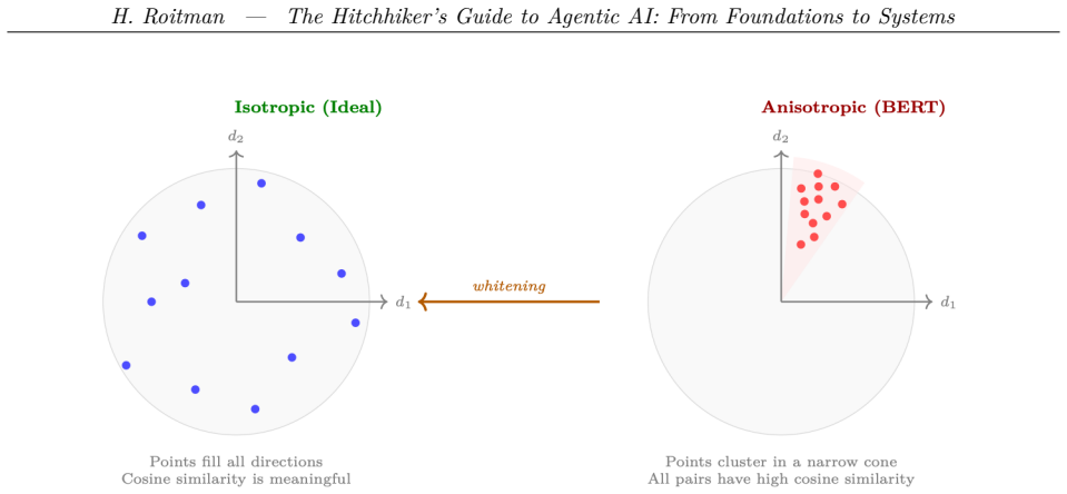
    Kawin Ethayarajh. How Contextual Are Contextualized Word Representations? Comparing the Geometry of BERT, ELMo, and GPT-2 Embeddings. InProceedings of the 2019 Conference on Empirical Methods in Natural Language Processing (EMNLP), 2019. URLhttps://arxiv. org/abs/1909.00512

  40. [41]

    Whitening Sentence Representations for Better Semantics and Faster Retrieval.arXiv Preprint arXiv:2103.15316, 2021

    Jianlin Su, Jiarun Cao, Weijie Liu, and Yangyiwen Ou. Whitening Sentence Representations for Better Semantics and Faster Retrieval.arXiv Preprint arXiv:2103.15316, 2021. URL https://arxiv.org/abs/2103.15316

  41. [42]

    Peters, and Arman Cohan

    Iz Beltagy, Matthew E. Peters, and Arman Cohan. Longformer: The Long-Document Trans- former.arXiv Preprint arXiv:2004.05150, 2020. URLhttps://arxiv.org/abs/2004.05150

  42. [43]

    Big Bird: Transformers for Longer Sequences

    Manzil Zaheer, Guru Guruganesh, Kumar Avinava Dubey, et al. Big Bird: Transformers for Longer Sequences. InAdvances in Neural Information Processing Systems (NeurIPS), 2020. URLhttps://arxiv.org/abs/2007.14062

  43. [44]

    LongT5: Efficient Text-to-Text Transformer for Long Sequences.Findings of the Association for Computational Linguistics: NAACL 2022,

    Mandy Guo, Joshua Ainslie, David Uthus, et al. LongT5: Efficient Text-to-Text Transformer for Long Sequences.Findings of the Association for Computational Linguistics: NAACL 2022,

  44. [45]

    URLhttps://arxiv.org/abs/2112.07916

  45. [47]

    RWKV: Reinventing RNNs for the Transformer Era.Findings of the Association for Computational Linguistics: EMNLP 2023, 2023

    Bo Peng, Eric Alcaide, Quentin Anthony, et al. RWKV: Reinventing RNNs for the Transformer Era.Findings of the Association for Computational Linguistics: EMNLP 2023, 2023. URL https://arxiv.org/abs/2305.13048

  46. [48]

    H2O: Heavy-Hitter Oracle for Efficient Generative Inference of Large Language Models

    Zhenyu Zhang, Ying Sheng, Tianyi Zhou, et al. H2O: Heavy-Hitter Oracle for Efficient Generative Inference of Large Language Models. InAdvances in Neural Information Processing Systems (NeurIPS), 2023. URLhttps://arxiv.org/abs/2306.14048

  47. [50]

    KIVI: A Tuning-Free Asymmetric 2bit Quantization for KV Cache

    Zirui Liu, Jiayi Yuan, Hongye Jin, et al. KIVI: A Tuning-Free Asymmetric 2bit Quantization for KV Cache. InInternational Conference on Machine Learning (ICML), 2024. URL https://arxiv.org/abs/2402.02750

  48. [51]

    Ring Attention with Blockwise Transformers for Near-Infinite Context

    Hao Liu, Matei Zaharia, and Pieter Abbeel. Ring Attention with Blockwise Transformers for Near-Infinite Context. InAdvances in Neural Information Processing Systems (NeurIPS), 2023. URLhttps://arxiv.org/abs/2310.01889

  49. [52]

    BLOOM: A 176B-Parameter Open-Access Multilingual Language Model

    BigScience Workshop. BLOOM: A 176B-Parameter Open-Access Multilingual Language Model. arXiv Preprint arXiv:2211.05100, 2023. URLhttps://arxiv.org/abs/2211.05100

  50. [53]

    MPT-7B: A New Standard for Open-Source, Commercially Usable LLMs.MosaicML Blog, 2023

    MosaicML. MPT-7B: A New Standard for Open-Source, Commercially Usable LLMs.MosaicML Blog, 2023. URLhttps://www.mosaicml.com/blog/mpt-7b

  51. [54]

    RoFormer: Enhanced Transformer with Rotary Position Embedding.Neurocomputing, 2024

    Jianlin Su, Murtadha Ahmed, Yu Lu, Shengfeng Pan, Wen Bo, and Yunfeng Liu. RoFormer: Enhanced Transformer with Rotary Position Embedding.Neurocomputing, 2024

  52. [55]

    YaRN: Efficient Context Window Extension of Large Language Models.arXiv Preprint arXiv:2309.00071, 2023

    Bowen Peng, Jeffrey Quesnelle, Honglu Fan, and Enrico Shao. YaRN: Efficient Context Window Extension of Large Language Models.arXiv Preprint arXiv:2309.00071, 2023

  53. [56]

    Smith, and Mike Lewis

    Ofir Press, Noah A. Smith, and Mike Lewis. Train Short, Test Long: Attention with Linear Biases Enables Input Length Generalization.ICLR, 2022

  54. [57]

    The Claude 3 Model Family: Opus, Sonnet, Haiku.Anthropic Technical Report,

    Anthropic. The Claude 3 Model Family: Opus, Sonnet, Haiku.Anthropic Technical Report,

  55. [58]

    URLhttps://www.anthropic.com/news/claude-3-family

  56. [59]

    Gemini 1.5: Unlocking Multimodal Understanding Across Millions of Tokens of Context.arXiv Preprint arXiv:2403.05530, 2024

    Google Gemini Team. Gemini 1.5: Unlocking Multimodal Understanding Across Millions of Tokens of Context.arXiv Preprint arXiv:2403.05530, 2024. URLhttps://arxiv.org/abs/ 2403.05530

  57. [61]

    URLhttps://arxiv.org/abs/2306.15595

  58. [62]

    Liu, Kevin Lin, John Hewitt, et al

    Nelson F. Liu, Kevin Lin, John Hewitt, et al. Lost in the Middle: How Language Models Use Long Contexts.Transactions of the Association for Computational Linguistics, 2024. URL https://arxiv.org/abs/2307.03172

  59. [63]

    Transformer Feed-Forward Layers Are Key-Value Memories

    Mor Geva, Roei Schuster, Jonathan Berant, and Omer Levy. Transformer Feed-Forward Layers Are Key-Value Memories. InProceedings of the 2021 Conference on Empirical Methods in Natural Language Processing (EMNLP), 2021

  60. [64]

    Jimmy Lei Ba, Jamie Ryan Kiros, and Geoffrey E. Hinton. Layer Normalization.arXiv Preprint arXiv:1607.06450, 2016. URLhttps://arxiv.org/abs/1607.06450

  61. [65]

    Root Mean Square Layer Normalization

    Biao Zhang and Rico Sennrich. Root Mean Square Layer Normalization. InAdvances in Neural Information Processing Systems (NeurIPS), 2019. URLhttps://arxiv.org/abs/1910.07467

  62. [66]

    The Llama 4 Herd: The Beginning of a New Era of Natively Multimodal AI.Meta AI Blog, 2025

    Meta AI. The Llama 4 Herd: The Beginning of a New Era of Natively Multimodal AI.Meta AI Blog, 2025. URLhttps://ai.meta.com/blog/llama-4-multimodal-intelligence/

  63. [67]

    Mistral Large 2.Mistral AI Blog, 2024

    Mistral AI. Mistral Large 2.Mistral AI Blog, 2024. URL https://mistral.ai/news/ mistral-large-2407/

  64. [68]

    DeepSeek-V3 Technical Report.arXiv Preprint arXiv:2412.19437, 2024

    DeepSeek-AI. DeepSeek-V3 Technical Report.arXiv Preprint arXiv:2412.19437, 2024. URL https://arxiv.org/abs/2412.19437

  65. [69]

    Efficient Streaming Language Models with Attention Sinks

    Guangxuan Xiao, Yuandong Tian, Beidi Chen, Song Han, and Mike Lewis. Efficient Streaming Language Models with Attention Sinks. InProceedings of the 12th International Conference on Learning Representations (ICLR), 2024. URLhttps://arxiv.org/abs/2309.17453. 581 H. Roitman — The Hitchhiker’s Guide to Agentic AI: From Foundations to Systems

  66. [70]

    Data Engineering for Scaling Language Models to 128K Context.arXiv Preprint arXiv:2402.10171, 2024

    Yao Fu, Rameswar Panda, Xinyao Niu, et al. Data Engineering for Scaling Language Models to 128K Context.arXiv Preprint arXiv:2402.10171, 2024. URL https://arxiv.org/abs/ 2402.10171

  67. [71]

    Mamba: Linear-Time Sequence Modeling with Selective State Spaces

    Albert Gu and Tri Dao. Mamba: Linear-Time Sequence Modeling with Selective State Spaces. InProceedings of the 41st International Conference on Machine Learning (ICML), 2024. URL https://arxiv.org/abs/2312.00752

  68. [72]

    Analyzing Multi- Head Self-Attention: Specialized Heads Do the Heavy Lifting, the Rest Can Be Pruned

    Elena Voita, David Talbot, Fedor Moiseev, Rico Sennrich, and Ivan Titov. Analyzing Multi- Head Self-Attention: Specialized Heads Do the Heavy Lifting, the Rest Can Be Pruned. In Proceedings of the 57th Annual Meeting of the Association for Computational Linguistics (ACL),

  69. [73]

    URLhttps://arxiv.org/abs/1905.09418

  70. [74]

    In-Context Learning and Induction Heads.Transformer Circuits Thread, 2022

    Catherine Olsson, Nelson Elhage, Neel Nanda, et al. In-Context Learning and Induction Heads.Transformer Circuits Thread, 2022. URL https://transformer-circuits.pub/ 2022/in-context-learning-and-induction-heads/index.html

  71. [76]

    URLhttps://arxiv.org/abs/2404.15574

  72. [77]

    A Multiscale Visualization of Attention in the Transformer Model

    Jesse Vig. A Multiscale Visualization of Attention in the Transformer Model. InProceedings of the 57th ACL: System Demonstrations, 2019. URLhttps://arxiv.org/abs/1906.05714

  73. [78]

    Quantifying Attention Flow in Transformers

    Samira Abnar and Willem Zuidema. Quantifying Attention Flow in Transformers. InProceedings of the 58th Annual Meeting of the Association for Computational Linguistics (ACL), 2020. URLhttps://arxiv.org/abs/2005.00928

  74. [79]

    Grad-SAM: Explaining Transformers via Gradient Self-Attention Maps

    Oren Barkan, Edan Hauon, Avi Caciularu, Ido Dagan, and Noam Koenigstein. Grad-SAM: Explaining Transformers via Gradient Self-Attention Maps. InProceedings of the 30th ACM International Conference on Information and Knowledge Management (CIKM), 2021. URL https://arxiv.org/abs/2104.13299

  75. [80]

    Sarthak Jain and Byron C. Wallace. Attention Is Not Explanation. InProceedings of the 2019 Conference of the North American Chapter of the Association for Computational Linguistics (NAACL), 2019. URLhttps://arxiv.org/abs/1902.10186

  76. [81]

    Sparse Autoencoders Find Highly Interpretable Features in Language Models

    Hoagy Cunningham, Aidan Ewart, Logan Riggs, Robert Huben, and Lee Sharkey. Sparse Autoencoders Find Highly Interpretable Features in Language Models. InProceedings of the 12th International Conference on Learning Representations (ICLR), 2024. URLhttps: //arxiv.org/abs/2309.08600

  77. [82]

    Towards Monosemanticity: Decom- posing Language Models with Dictionary Learning.Transformer Circuits Thread, 2023

    Trenton Bricken, Adly Templeton, Joshua Batson, et al. Towards Monosemanticity: Decom- posing Language Models with Dictionary Learning.Transformer Circuits Thread, 2023. URL https://transformer-circuits.pub/2023/monosemantic-features/index.html

  78. [83]

    Scaling Monosemanticity: Extracting Interpretable Features from Claude 3 Sonnet.Transformer Circuits Thread, 2024

    Adly Templeton, Tom Conerly, Jonathan Marcus, et al. Scaling Monosemanticity: Extracting Interpretable Features from Claude 3 Sonnet.Transformer Circuits Thread, 2024. URL https://transformer-circuits.pub/2024/scaling-monosemanticity/index.html

  79. [84]

    Natural Language Autoencoders: Interpreting Neural Networks with Natural Language Descriptions.Anthropic Research Blog, 2026

    Anthropic. Natural Language Autoencoders: Interpreting Neural Networks with Natural Language Descriptions.Anthropic Research Blog, 2026. URLhttps://www.anthropic.com/ research/natural-language-autoencoders

  80. [85]

    Rumelhart, Geoffrey E

    David E. Rumelhart, Geoffrey E. Hinton, and Ronald J. Williams. Learning Representations by Back-Propagating Errors.Nature, 1986. URLhttps://doi.org/10.1038/323533a0

Showing first 80 references.