Polynomial Neural Sheaf Diffusion: A Spectral Filtering Approach on Cellular Sheaves
Pith reviewed 2026-05-21 17:33 UTC · model grok-4.3
The pith
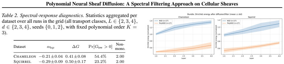
A polynomial in the normalized sheaf Laplacian lets neural sheaf networks reach state-of-the-art accuracy on heterophilic graphs using only diagonal restriction maps.
A machine-rendered reading of the paper's core claim, the machinery that carries it, and where it could break.
Core claim
A degree-K polynomial propagation operator on a spectrally rescaled and normalized sheaf Laplacian, obtained as a convex mixture of K+1 orthogonal polynomial responses and computed by three-term recurrence, supplies a stable, explicit multi-hop filter for cellular-sheaf diffusion models. This operator attains new state-of-the-art results on standard and heterophilic benchmarks while permitting the use of diagonal restriction maps only, thereby decoupling accuracy from stalk dimension and removing the need for repeated Laplacian rebuilds or dense per-edge maps.
What carries the argument
The polynomial propagation operator formed as a convex mixture of orthogonal polynomial basis responses on a spectrally rescaled normalized sheaf Laplacian and evaluated by stable three-term recurrence.
If this is right
- Single-layer models obtain explicit K-hop neighborhoods independent of stalk dimension.
- Training stability improves through convex coefficient mixtures and spectral rescaling.
- Runtime and memory scale with graph size rather than with stalk dimension.
- Heterophily handling no longer requires complex learned restriction maps on every edge.
- The approach inverts the prior trend that larger stalks and denser maps were needed for competitive performance.
Where Pith is reading between the lines
- The success with diagonal maps alone suggests that most heterophily correction is supplied by the learned spectral filter rather than by the geometry of the restriction maps.
- The same polynomial construction could be transferred to other topological or geometric message-passing schemes that currently rely on expensive per-edge transformations.
- Because the recurrence avoids repeated matrix factorizations, the method may extend naturally to time-varying or streaming graph settings where the underlying sheaf changes.
- Testing whether the orthogonal polynomial basis can be replaced by other stable families while preserving the convex-mixture guarantee would clarify how much of the reported gain is tied to the specific basis choice.
Load-bearing premise
A convex mixture of orthogonal polynomial responses on a spectrally rescaled operator remains stable and expressive for arbitrary cellular sheaves without requiring dense per-edge maps or frequent Laplacian rebuilds.
What would settle it
A controlled experiment on a heterophilic benchmark in which PolyNSD with diagonal restriction maps fails to match or exceed the accuracy of prior sheaf diffusion models that use full dense maps while also showing no reduction in memory or runtime.
Figures


read the original abstract
Sheaf Neural Networks equip graph structures with a cellular sheaf: a geometric structure which assigns local vector spaces (stalks) and a linear learnable restriction/transport maps to nodes and edges, yielding an edge-aware inductive bias that handles heterophily and limits oversmoothing. However, common Neural Sheaf Diffusion implementations rely on SVD-based sheaf normalization and dense per-edge restriction maps, which scale with stalk dimension, require frequent Laplacian rebuilds, and yield brittle gradients. To address these limitations, we introduce Polynomial Neural Sheaf Diffusion (PolyNSD), a new sheaf diffusion approach whose propagation operator is a degree-K polynomial in a normalised sheaf Laplacian, evaluated via a stable three-term recurrence on a spectrally rescaled operator. This provides an explicit K-hop receptive field in a single layer (independently of the stalk dimension), with a trainable spectral response obtained as a convex mixture of K+1 orthogonal polynomial basis responses. PolyNSD enforces stability via convex mixtures, spectral rescaling, and residual/gated paths, reaching new state-of-the-art results on both homophilic and heterophilic benchmarks, inverting the Neural Sheaf Diffusion trend by obtaining these results with just diagonal restriction maps, decoupling performance from large stalk dimension, while reducing runtime and memory requirements.
Editorial analysis
A structured set of objections, weighed in public.
Referee Report
Summary. The manuscript introduces Polynomial Neural Sheaf Diffusion (PolyNSD), a spectral filtering method for cellular sheaves on graphs. The propagation operator is defined as a degree-K polynomial in a normalized sheaf Laplacian, evaluated via three-term recurrence on a spectrally rescaled version of the operator. The trainable spectral response is formed as a convex mixture of K+1 orthogonal polynomial basis responses. The method uses only diagonal restriction maps, claims an explicit K-hop receptive field independent of stalk dimension, enforces stability through convex mixtures, spectral rescaling, and residual/gated paths, and reports new state-of-the-art results on both homophilic and heterophilic benchmarks while reducing runtime and memory requirements compared to prior Neural Sheaf Diffusion approaches.
Significance. If the stability guarantees hold under learnable diagonal restriction maps and the reported benchmark gains prove robust to hyperparameter choices, this work would offer a computationally efficient spectral alternative for sheaf neural networks that decouples performance from stalk dimension and provides an explicit receptive field without dense per-edge maps. The combination of orthogonal polynomial bases with convex mixtures and rescaling is a concrete advance over SVD-based normalization in prior work, and the empirical inversion of the trend toward large stalks is noteworthy if reproducible.
major comments (2)
- [§3.2] §3.2 (Propagation Operator): The spectral rescaling factor applied to the sheaf Laplacian before the three-term recurrence is not stated to be fixed at initialization or recomputed per forward pass. With trainable diagonal restriction maps (Eq. (2)), each gradient update can shift the eigenvalues of the resulting Laplacian (Eq. (3)), potentially moving the spectrum outside the design interval assumed for stability of the orthogonal polynomial recurrence and convex mixture. This directly affects the central claim that stability is enforced without frequent Laplacian rebuilds.
- [§5] §5 (Experiments): The SOTA results on heterophilic benchmarks are presented without an ablation isolating the contribution of the polynomial degree K versus the choice of rescaling factor (both listed as free parameters in the abstract). The performance gains could therefore be driven by hyperparameter selection rather than the architectural innovations, weakening the claim that diagonal restriction maps alone suffice to decouple performance from stalk dimension.
minor comments (2)
- [§3.3] The notation for the convex mixture weights in the spectral response (around Eq. (7)) should be introduced earlier and tied explicitly to the stability argument in the abstract.
- [§5] Table 1 and Table 2 would benefit from an additional column reporting the chosen polynomial degree K and rescaling factor for each dataset to aid reproducibility.
Simulated Author's Rebuttal
We thank the referee for the constructive feedback on our manuscript. The comments help clarify key aspects of the stability mechanism and experimental validation. We respond to each major comment below and indicate the revisions we plan to incorporate.
read point-by-point responses
-
Referee: [§3.2] §3.2 (Propagation Operator): The spectral rescaling factor applied to the sheaf Laplacian before the three-term recurrence is not stated to be fixed at initialization or recomputed per forward pass. With trainable diagonal restriction maps (Eq. (2)), each gradient update can shift the eigenvalues of the resulting Laplacian (Eq. (3)), potentially moving the spectrum outside the design interval assumed for stability of the orthogonal polynomial recurrence and convex mixture. This directly affects the central claim that stability is enforced without frequent Laplacian rebuilds.
Authors: We thank the referee for this observation. The spectral rescaling factor is computed once at initialization from the eigenvalues of the initial normalized sheaf Laplacian (ensuring the spectrum lies in the design interval for the chosen orthogonal polynomial basis) and is held fixed during training. This design choice avoids per-forward-pass recomputation and the associated Laplacian rebuilds. While diagonal restriction maps are trainable, the combination of convex mixtures of polynomial responses, spectral rescaling, and residual/gated paths (as analyzed in Section 4) is intended to preserve stability bounds. We acknowledge that the manuscript does not explicitly state the fixed-at-initialization choice. We will revise §3.2 to make this explicit and add a brief remark justifying boundedness under diagonal updates. revision: yes
-
Referee: [§5] §5 (Experiments): The SOTA results on heterophilic benchmarks are presented without an ablation isolating the contribution of the polynomial degree K versus the choice of rescaling factor (both listed as free parameters in the abstract). The performance gains could therefore be driven by hyperparameter selection rather than the architectural innovations, weakening the claim that diagonal restriction maps alone suffice to decouple performance from stalk dimension.
Authors: We appreciate the suggestion to isolate these factors. Our reported results already include comparisons across stalk dimensions showing that diagonal restriction maps suffice for strong performance (in contrast to prior Neural Sheaf Diffusion methods), and the rescaling is chosen to align with the polynomial degree K for stable approximation. However, we did not present a dedicated ablation varying K independently of the rescaling strategy. To strengthen the experimental section and support the decoupling claim, we will add an ablation study in the revised version that reports performance for different K values with fixed rescaling and vice versa on the heterophilic benchmarks. This will help demonstrate that gains are attributable to the polynomial filtering approach rather than isolated hyperparameter choices. revision: yes
Circularity Check
No circularity in operator definition or stability claims
full rationale
The paper constructs PolyNSD by defining the propagation operator explicitly as a degree-K polynomial in a spectrally rescaled normalized sheaf Laplacian, evaluated via three-term recurrence with a convex mixture of orthogonal polynomial bases. This is a direct architectural choice with stability enforced by the mixture, rescaling, and residual/gated paths rather than any fitted quantity renamed as a prediction or any self-referential derivation. No load-bearing self-citation for uniqueness theorems, no ansatz smuggled via prior work, and no reduction of the central claim to its own inputs by construction. Empirical SOTA results are reported separately on benchmarks and do not enter the operator definition.
Axiom & Free-Parameter Ledger
free parameters (2)
- polynomial degree K
- spectral rescaling factor
axioms (1)
- domain assumption The normalized sheaf Laplacian admits a stable polynomial approximation via three-term recurrence for any cellular sheaf.
Forward citations
Cited by 1 Pith paper
-
Deep Neural Sheaf Diffusion
DNSD replaces the sheaf Laplacian with a sheaf adjacency operator to maintain informative signals in deep layers, outperforming GNN and NSD baselines on long-range synthetic and real graph tasks.
Reference graph
Works this paper leans on
-
[1]
Hence, we get: p(m)(LF) ∥·∥2 − − − − → m→∞ f(L F)(26) This shows both that f(L F) is the operator-theoretic limit of p(m)(LF) and that the operator is independent of the particular approximating sequence (p(m))m, since any two such sequences will converge to the same diagonal f(Λ) entrywise on the eigenvalues. Step 4: Operator norm identity.We now prove t...
work page 2019
-
[2]
Extremal Property and Uniform Bound.First-kind Chebyshev polynomials satisfy Tk(ξ) = cos(karccosξ),|ξ| ≤1 , and hence: |Tk(ξ)| ≤1for allξ∈[−1,1], k≥0(37) This extremal/minimax propertyonlyholds on[−1,1]. For|ξ|>1, Chebyshev polynomials grow exponentially: Tk(ξ) = cosh karcosh|ξ| ,|ξ|>1(38) so |Tk(ξ)| behaves like c(ξ)ρ(ξ) k with ρ(ξ)>1 . If we were to app...
-
[3]
Transferring Scalar Approximation Bounds to Operators.All classical Chebyshev approximation results, are stated for functions on [−1,1] . What we want in PolyNSD is anoperatorapproximation of a spectral multiplier f(L), with σ(L)⊂[0, λ max]. The affine map ξ(λ) = 2 λmax λ−1 identifies [0, λmax] with [−1,1] . We approximate ˜f(ξ) := f( λmax 2 (ξ+ 1)) by a ...
-
[4]
In the eigenbasis ofL, the linear operatorx7→p( eL)x+α hphhp has per-eigenvalue multiplier: m(λ) =p 2λ λmax −1 +α hp 1− λ λmax , λ∈σ(L)(77) In particular, if αhp >0 and p(ξ)≥0 for all ξ∈[−1,1] , then m(λ)>0 for all λ∈[0, λ max), so no non-harmonic mode (λ >0withλ < λ max) can be annihilated
-
[5]
Proof.We treat the two claims separately
The full mappingT:x7→x + satisfies the global Lipschitz bound: ∥T(x)−T(y)∥ 2 ≤ h 1 +∥tanhε∥ ∞ + Lip(ϕ) 1 + 2|αhp| i ∥x−y∥ 2,(78) i.e.Tis Lipschitz with constant at most:L T ≤ 1 +∥tanhε∥ ∞ + Lip(ϕ) 1 + 2|αhp| . Proof.We treat the two claims separately. (1) Spectral Multiplier of the High-pass Skip. SinceeL is an affine function of L, we have LeL= eLL and t...
work page 2022
-
[6]
Draw class prototypesv k ∼ U([0,1] ndata)fork= 1, . . . , n c
-
[7]
Define a fixed non-linear mapf:R nh →R ndata as the sine–cosine embedding of the(nh −1)-sphere. We sample angles θ0, . . . , θnh−3 ∼ U([0, π]) and θnh−2 ∼ U([0,2π)) , construct s∈S nh−1 via standard hyperspherical coordinates, and setz=f(θ)after truncating/tiling to lengthn data
-
[8]
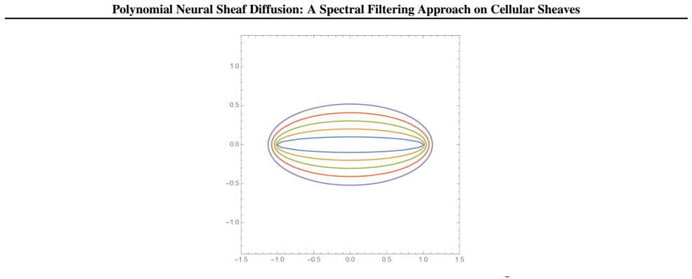
For a node of class k, we sample θ as above and set the raw feature xraw =v k ⊙f(θ) , where ⊙ denotes element-wise multiplication, yielding an ellipsoidal shell per class
-
[9]
We centre features to enforce a shared expected value across classesµ= 1 N PN i=1 xraw,i,˜xi =x raw,i −µ
-
[10]
Gaussian noiseϵ i ∼ N(0, σ 2I)and optionally rescalex i = ˜xi +ϵ i
Finally, we add i.i.d. Gaussian noiseϵ i ∼ N(0, σ 2I)and optionally rescalex i = ˜xi +ϵ i. Graph Generation: Ring–rewire with Class-aware Mixing.Connectivity is generated independently of features and controlled by the heterophily indexhet. The graph generation process consists in:
-
[11]
Assign classes almost uniformly so that|C k| ≈N/n c
-
[12]
Build a regular ring lattice of degreeK, beingE= (i, j) : 0<min(|i−j|, N−|i−j|)≤K/2
-
[13]
Define the class–transition matrix Rc = (1−het)I nc + het nc−1 (11⊤ −I nc) so that Pr(same class) = 1−het and each different class has probabilityhet/(n c −1)
-
[14]
For each node i and each of its K/2 “rightmost” edges, rewire with probability p, we sample a target class c′ ∼ Categorical (Rc)ci,: , where ci is the class of node i and choose j uniformly among nodes in class c′ that are not i and not already adjacent to i, and replace the endpoint with j. We then de-duplicate multi-edges and remove self-loops. The aver...
work page 2024
discussion (0)
Sign in with ORCID, Apple, or X to comment. Anyone can read and Pith papers without signing in.